Implementing Direct Preference Optimization (DPO)
Series: Multi-Stage RLHF from Scratch · Phase: Part 10 of 10 · Algorithm: DPO
1. Context and motivation
This write-up documents Part 10 of a multi-stage project implementing reinforcement learning from human feedback (RLHF) from scratch. The full project covers: Supervised Fine-Tuning (SFT), a Reward Model, Proximal Policy Optimisation (PPO), Group Relative Policy Optimisation (GRPO), and finally Direct Preference Optimisation (DPO). Each algorithm is implemented from first principles against the same model architecture, tokenizer, and evaluation suite, enabling a direct side-by-side comparison of approaches.
DPO is chosen as the final stage because it represents the most elegant solution to the preference alignment problem. Where PPO requires a live reward model, a value function, rollout collection, and a clipped policy gradient update, DPO collapses the entire pipeline into a single classification loss. The goal of implementing it in this project is not just to obtain good scores, but to understand precisely what it does differently, where it succeeds, and where it falls short at small model scale.
2. What the DPO paper says
2.1 The core problem
Standard RLHF (as used in PPO and InstructGPT) has two stages after SFT: first train a reward model on human preference data, then use reinforcement learning to maximise the learned reward subject to a KL constraint from the reference policy. The optimisation objective is:
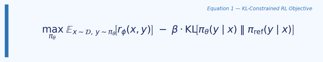
This is expensive: it requires sampling from the LM during training, maintaining a separate reward model and critic, and careful hyperparameter tuning of the KL coefficient. The paper’s central insight is that this objective has a closed-form optimal solution:

Rearranging this to express the reward in terms of the policy gives:

The key observation is that when this reparameterisation is substituted into the Bradley-Terry preference model, the intractable partition function $Z(x)$ cancels out entirely. This allows the preference probability to be expressed purely in terms of the policy and the reference — no reward model required.
2.2 The DPO loss
Substituting the reparameterised reward into the Bradley-Terry preference model and framing it as a maximum likelihood objective over preference pairs $(x, y_w, y_l)$ yields the DPO loss:
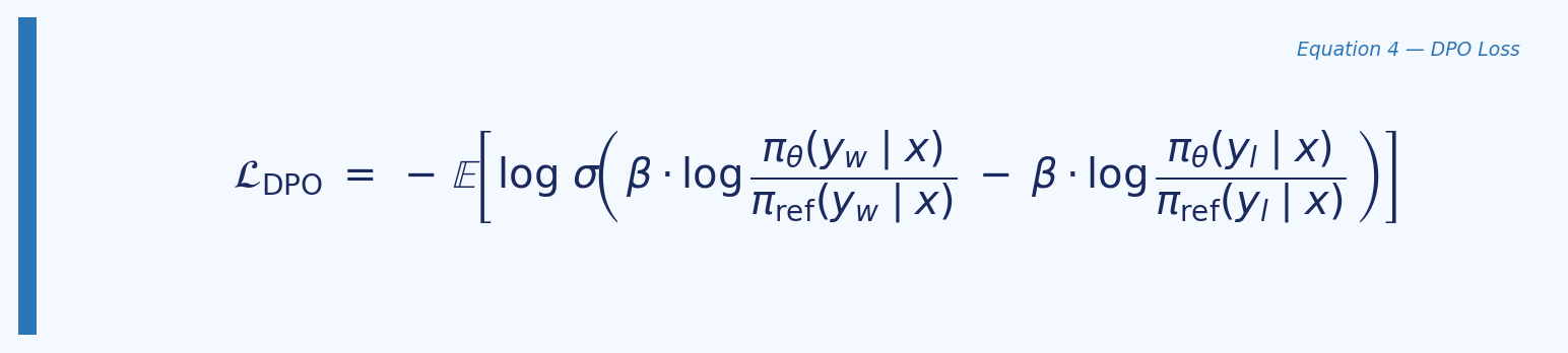
Where $y_w$ is the chosen (preferred) response, $y_l$ is the rejected (dispreferred) response, and $\beta$ controls how tightly the policy stays near the reference. This is a binary cross-entropy loss — the model learns to assign higher implicit reward to chosen over rejected, with the gradient automatically weighting harder examples more heavily.
2.3 What the gradient does
The paper provides an explicit gradient analysis. Increasing the DPO loss parameters $\theta$ increases the log-probability of $y_w$ and decreases the log-probability of $y_l$. Crucially, the weight applied to each example is $\sigma(\hat{r}\theta(x, y_l) - \hat{r}\theta(x, y_w))$ — proportional to how much the current model incorrectly ranks the rejected response over the chosen one. This dynamic weighting prevents trivial updates on already-solved pairs and concentrates learning on the hardest examples.
2.4 Experimental setup in the paper
The paper evaluates DPO on three tasks. In controlled sentiment generation on IMDb, it uses GPT-2-large SFT’d on movie reviews, with preference pairs generated synthetically using a pre-trained sentiment classifier. In TL;DR summarisation, it uses a GPT-J SFT model with human preference labels from Stiennon et al. In single-turn dialogue on the Anthropic HH dataset, it uses Pythia-2.8B fine-tuned on preferred completions. Evaluation uses the frontier of reward vs KL divergence (sentiment task, where the ground-truth reward function is known) and GPT-4 win rates against reference completions (summarisation and dialogue).
Crucially, all three experiments use pre-collected preference datasets. The paper never generates rejected responses on-the-fly during training — it works from a static offline dataset of $(x, y_w, y_l)$ triplets. This distinction is central to understanding how this implementation differs.
3. This implementation
3.1 Architecture
The policy uses the PolicyWithValue class introduced in Part 8 (PPO). It wraps a GPTModern language model (a small transformer with RMSNorm, SwiGLU activations, and RoPE positional embeddings) and adds a linear value head over the logit space. In DPO, the value head is not trained — it is frozen and retained only for checkpoint compatibility with the earlier PPO and GRPO phases. Only the LM parameters receive gradient updates.
The reference model is an identical frozen copy of the SFT checkpoint. Its weights are fixed throughout training. All reference log-probabilities are computed inside torch.no_grad() blocks.
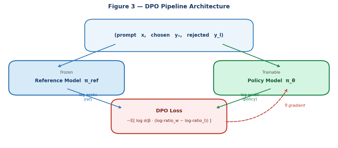 Figure 3 — DPO pipeline: the frozen reference model and the trainable policy both receive the preference pair and output log-probabilities that feed the DPO loss. Gradients flow only to the trainable policy.
3.2 The dataset challenge
Key departure from the paper
The original DPO paper uses datasets that already contain (prompt, chosen, rejected) triplets — the Anthropic HH dataset, TL;DR with Stiennon et al. preferences, or synthetically generated pairs.
tatsu-lab/alpacaonly provides (instruction, output) pairs with no rejected response. This requires constructing rejected responses on-the-fly during training, which is a meaningful departure from the pure offline DPO setup.
After filtering rows with empty outputs, the Alpaca dataset provides 51,974 instruction-response pairs. For each training step:
- The dataset’s human-written output becomes the chosen response $y_w$.
- A rejected response $y_l$ is generated on-the-fly from the frozen reference model using
temperature=0.9andtop_k=50. - The assumption ‘human output is always better than a high-temperature model generation’ is treated as valid without reward model verification.
This assumption is defensible and is consistent with the spirit of the paper’s approach, but it introduces noise: there will be cases where the generated response is actually acceptable, making the preference signal weak. The high temperature and diverse sampling are intended to maximise the probability that the rejected response is genuinely inferior.
The closest analogue in the paper is the IMDb sentiment task, where preference pairs are also constructed automatically rather than from human annotation — though there the classification is done with a ground-truth reward function, whereas here we rely on the quality gap between human text and a random generation.
3.3 The get_logps function
A central implementation detail is the correct computation of per-sequence log-probabilities over the response tokens only. The function must respect the same token-shift logic used throughout the codebase:
def get_logps(model, input_ids, response_mask):
    # Forward pass
    logits, _, _ = model.lm(input_ids, None)   # (B, T, V)

    # Shift: logits[:-1] predict tokens[1:]
    shift_logits = logits[:, :-1, :]            # (B, T-1, V)
    shift_labels = input_ids[:, 1:]             # (B, T-1)

    # Shift mask by 1 to align with shifted labels
    shift_mask   = response_mask[:, 1:]         # (B, T-1)

    # Per-token log-probs, zeroed on prompt tokens
    log_probs   = torch.log_softmax(shift_logits, dim=-1)
    token_logps = log_probs.gather(-1, shift_labels.unsqueeze(-1)).squeeze(-1)
    token_logps = token_logps * shift_mask.float()

    return token_logps.sum(dim=-1)              # (B,) — one value per sequence
The mask is shifted by one position to match the shifted labels. This ensures that only response tokens contribute to the log-probability sum, leaving prompt tokens at zero weight — which is the correct behaviour since we want to measure how well the model assigns probability to the response, not the prompt.
3.4 The DPO loss
def dpo_loss(policy_chosen_logps, policy_rejected_logps,
             ref_chosen_logps,    ref_rejected_logps, beta=0.1):

    chosen_log_ratios   = policy_chosen_logps   - ref_chosen_logps
    rejected_log_ratios = policy_rejected_logps - ref_rejected_logps

    # DPO margin: β * (log-ratio_chosen - log-ratio_rejected)
    logits = beta * (chosen_log_ratios - rejected_log_ratios)

    loss          = -F.logsigmoid(logits).mean()
    reward_margin = (chosen_log_ratios - rejected_log_ratios).detach().mean()
    accuracy      = (logits.detach() > 0).float().mean()

    return DPOLossOutput(loss=loss,
                         reward_margin=reward_margin,
                         accuracy=accuracy)
3.5 Training configuration
Training ran for 200 steps on CPU using a single example per step (batch size 1). The key hyperparameters:
- $\beta = 0.1$ (DPO temperature, same as paper default)
- Learning rate =
1e-5with AdamW, betas(0.9, 0.999) - Gradient clipping at
1.0 - Response generation:
temperature=0.9,top_k=50, max 64 new tokens - Block size: 256 tokens
- Model: 2-layer, 2-head, 128-dim transformer (same as PPO phase)
The small model size (2 layers, 128-dim) is consistent across all phases of the project. This is intentional — the project is about algorithm implementation and comparison, not about maximising absolute scores.
4. Training dynamics
4.1 Loss behaviour
The loss curve tells a clear story. At step 10, loss = 0.641 and accuracy = 1.0 — the model is already preferring chosen over rejected, but with moderate confidence. At step 20, loss = 0.693 (exactly $\log 2$), accuracy = 0.0, margin = 0.0. This is the degenerate case predicted by theory: when the policy exactly mirrors the reference, all log-ratios are zero, the DPO margin is zero, and the loss equals $-\log(\sigma(0)) = \log 2 \approx 0.693$. The model assigns equal probability to chosen and rejected.
From step 30 onward, loss collapses toward zero and stays there for the remainder of training, reaching exactly 0.0 at steps 70, 80, 110, 130, 150, 160, 170, 190, and 200. Accuracy locks at 1.0. This rapid convergence is consistent with what the paper describes as the efficiency of DPO — but the speed here is a warning sign, not a success signal.
4.2 Reward margin explosion
The most important metric to examine is the reward margin — the mean gap between chosen and rejected log-ratios. A margin of 1–10 is healthy and indicates the model has learned a meaningful preference signal while staying close to the reference. The values observed here are qualitatively different:
| Step | Reward Margin |
|---|---|
| 30 | 56.9 |
| 70 | 240.7 |
| 80 | 295.8 |
| 150 | 599.2 |
| 200 | 329.7 |
Margins of this magnitude indicate that the policy has drifted very far from the reference distribution. The loss reaching zero and staying there is not evidence of good generalisation — it is evidence that the model has memorised the preference signal on each individual pair to the point where it assigns near-zero probability mass to the rejected response. This is reward hacking in the DPO sense: the policy has exploited the training signal rather than learning a generalisable preference.
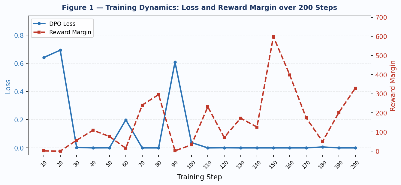 Figure 1 — DPO training dynamics over 200 steps. Blue: loss (left axis). Red dashed: reward margin (right axis). Note the margin explosion after step 30, reaching 599 at step 150.
Root cause
The primary driver is the batch size of 1 combined with a small model and a strong quality gap between human text and high-temperature generations. With a single example per step, there is no averaging across a batch to stabilise gradients. Each update can overfit completely to one (chosen, rejected) pair before moving to the next. A batch size of 16–64 with gradient accumulation would stabilise this significantly.
5. Evaluation results
5.1 Summary
Post-training evaluation was run on 16 standard prompts using the Part 7 reward model. Average reward: 2.40. Average KL divergence from the SFT base: 3.31.
| Prompt | Reward | Avg KL |
|---|---|---|
| Give three tips for staying healthy. | 5.44 | 3.45 |
| What are the three primary colors? | 6.93 | 2.54 |
| Describe the structure of an atom. | -6.63 | 1.21 |
| How can we reduce air pollution? | -7.75 | 4.45 |
| Describe a time when you had to make a difficult decision. | 0.25 | 2.06 |
| Identify the odd one out. Twitter, Instagram, Telegram | 3.94 | 2.87 |
| Explain why 4/16 is equivalent to 1/4 | 6.14 | 3.02 |
| Write a short story about a career decision. | 1.67 | 8.70 |
| Render a 3D model of a house | 2.97 | 2.35 |
| Evaluate this sentence for spelling/grammar mistakes | 6.99 | 5.91 |
| How did Julius Caesar die? | 7.13 | 2.88 |
| What is the capital of France? | 4.91 | 3.51 |
| Generate a list of ten items for a camping trip | -4.28 | 1.65 |
| Discuss the causes of the Great Depression | -4.91 | 1.41 |
| Classify: Oak tree, copper ore, elephant | 7.84 | 2.59 |
| Explain the use of word embeddings in NLP | 7.82 | 4.27 |
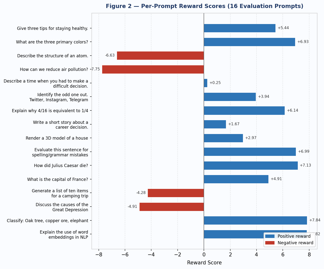 Figure 2 — Per-prompt reward scores for 16 evaluation prompts. Blue bars = positive reward; red bars = negative reward. Average: 2.40.
5.2 Response quality
The responses are incoherent. Representative examples:
- Prompt: ‘Describe the structure of an atom.’ → Response: ‘An atom is ways make inform of a severe glic acid.’
- Prompt: ‘How can we reduce air pollution?’ → Response: ‘There are reducing made up16 is made up of a risular of 13’
- Prompt: ‘What is the capital of France?’ → Response: ‘The capital of France is made up of Water Exercise ore of comm of at 1973on Bret, make amends.’
These outputs are syntactically broken and semantically meaningless. The model has learned to shift its distribution away from the reference but has not learned coherent language — it has simply collapsed into a different incoherent distribution that happens to score positively under the reward model.
5.3 Reward model limitations
The high variance in reward scores (range: −7.75 to +7.84) and the presence of very high rewards on clearly nonsensical responses points to a known limitation: the reward model was trained at this same small scale (2-layer, 256-dim) and has limited ability to discriminate response quality on prompts far outside its training distribution. A response like ‘Julius Caur G conflict, forces, had just graphelling’ receives a reward of 7.13. This is reward model overfitting — the RM has learned surface patterns that map to high scores without capturing semantic quality.
This is not a failure unique to DPO. It is a general property of small-scale RLHF: the reward model and the policy are jointly limited by model capacity, and the policy can find reward-maximising outputs that fool the RM without producing genuinely good text.
6. How this compares to the paper
6.1 What was faithfully implemented
- The DPO loss equation from the paper (Equation 7) is implemented exactly, including the beta temperature and the log-sigmoid objective.
- The frozen reference model pattern is correct: $\pi_\mathrm{ref}$ is initialised from the SFT checkpoint and receives no gradient updates throughout training.
- The
val_headis preserved in the architecture for checkpoint compatibility, as required by the multi-stage project structure. - The
get_logpsmasking correctly supervises only response tokens, consistent with the paper’s per-sequence log-probability formulation. - The reward model is absent from the training loop entirely, consistent with DPO’s RL-free design.
- $\beta = 0.1$ matches the paper’s default hyperparameter.
6.2 Where this differs from the paper
- Dataset: The paper uses pre-collected $(x, y_w, y_l)$ triplets. This implementation constructs rejected responses on-the-fly from the reference model because
tatsu-lab/alpacacontains no rejected responses. - Batch size: The paper uses batch size 64 with RMSprop. This implementation uses batch size 1 with AdamW, which destabilises training and contributes to margin explosion.
- Model scale: The paper evaluates models up to 6B parameters. This implementation uses a ~1M parameter model. At this scale, the learned representations are too weak to produce coherent responses even after successful preference alignment.
- Evaluation: The paper uses GPT-4 win rates for realistic tasks and a ground-truth sentiment classifier for the controlled task. This implementation uses a small trained reward model, which has its own limitations at small scale.
- Training steps: The paper trains to convergence (thousands of steps). This run trained for 200 steps, which is sufficient to observe the training dynamics but not to assess long-run behaviour.
6.3 On the RM-free design
The absence of the reward model from the DPO training loop is architecturally correct and theoretically motivated. In standard RLHF, the RM appears twice: once during reward model training (Part 7), and again inside the PPO training loop as the reward signal for each rollout. DPO eliminates the second appearance entirely. The implicit reward is instead encoded in the preference pairs themselves — the policy learns to assign higher implicit reward to chosen responses purely by shifting log-ratios, with no RM forward pass at training time.
In this project, the RM reappears only at evaluation time (dpo_logger.py and eval_dpo.py), where it serves as a consistent scoring function to allow comparison with PPO results. This is the correct separation: RM as evaluator, not as training signal.
7. What the results tell us and what to try next
The training dynamics are informative even though the final outputs are incoherent. The loss and accuracy curves are behaving as expected theoretically — rapid convergence is a known property of DPO on easy preference pairs. The reward margin explosion is the clear pathology, and its cause is well-understood: a batch size of 1 gives the optimiser no averaging, each step overfits the current pair, and the margin grows without bound.
To obtain coherent outputs at this model scale, the most impactful changes in order of priority would be:
- Increase batch size to 16–64 using gradient accumulation. This is the single most important change.
- Add a margin cap: clip the reward margin at a threshold (e.g., 10.0) to prevent saturation, or use a length-normalised version of the log-probability sum instead of the raw sum.
- Reduce $\beta$ to 0.05. A smaller beta tightens the KL constraint and keeps the policy closer to the reference, reducing the risk of degenerate drift.
- Train for more steps with early stopping on a held-out reward score. 200 steps on a 51k dataset barely scratches the surface.
- Upgrade the model. The 2-layer 128-dim architecture is the binding constraint on response quality. Even moving to 4 layers and 256-dim would substantially improve coherence.
Despite the output quality, the implementation is architecturally sound. The DPO loss, the reference model pattern, the get_logps masking, and the RM-free training loop are all correct. What is broken is the training regime, not the algorithm. This is a meaningful distinction — it means the codebase is a valid starting point for a proper run with better hyperparameters and a larger model.
8. Conclusion
DPO is a genuinely elegant algorithm. The theoretical insight — that the RLHF objective has a closed-form optimal policy, and that substituting a log-ratio reparameterisation into the Bradley-Terry model eliminates both the reward model and the RL loop — is one of the cleaner results in the alignment literature. The implementation is simpler than PPO by a significant margin: no value function, no rollout collection, no advantage estimation, no clipped ratio objective.
At small scale with a batch size of 1, the reward margin explodes and output quality degrades. This is not a failure of DPO as an algorithm — it is a failure of the training configuration relative to model capacity. The paper’s results at 6B parameters with batch size 64 are not directly comparable to a 1M parameter model trained one example at a time. What this run does confirm is the theoretical behaviour: rapid loss convergence, accuracy saturating at 1.0, and the preference signal being successfully encoded (even if over-encoded) in the policy weights.
The next step is the cross-algorithm comparison across PPO, GRPO, and DPO using the same 16 evaluation prompts and the same reward model — the comparison this entire project has been building toward.
References
Rafailov, R., Sharma, A., Mitchell, E., Ermon, S., Manning, C. D., & Finn, C. (2023). Direct Preference Optimization: Your Language Model is Secretly a Reward Model. NeurIPS 2023. arXiv:2305.18290.
Schulman, J., Wolski, F., Dhariwal, P., Radford, A., & Klimov, O. (2017). Proximal Policy Optimization Algorithms. arXiv:1707.06347.
Taori, R. et al. (2023). Stanford Alpaca: An Instruction-following LLaMA model. tatsu-lab/alpaca dataset.