From Pixels to Labels: Building a Satellite Image Segmentation Model
I spent the last year building language models. Transformers, attention, and RLHF: I knew that world well. Then someone handed me an image segmentation task and I realized I had a blind spot the size of a continent.
This post documents what I learned and built, starting from what segmentation actually is, why the standard approach breaks down with limited labels, and how a custom loss function fixes it.
If you already know what semantic segmentation is, skip to the section on the loss function. If you are coming from NLP like I was, start here.
Classification, detection, segmentation: three questions about the same image
Before I get into segmentation, it helps to place it next to the other two things a vision model can do with the same photograph: classify it, or detect objects in it. Each one answers a different question, and each one throws away information the other two keep.
Classification answers one question for the whole image: what is the dominant thing here. Feed a network a photo of a farm and it says “field,” one label, done. It doesn’t say where the field is in the frame or where it ends. For a lot of problems that’s enough. For a satellite tile with five different land types sitting next to each other, it tells you almost nothing.
Detection answers a better question: what objects are here, and roughly where. Run a detector on that same photo and you get boxes, one around a barn, one around a tractor, each with a label and a confidence score. Better, but a box is a crude shape. A rectangle drawn around a barn also covers the driveway, the grass, and half the field behind it.
Segmentation answers the most demanding version of the question: for every pixel, what does it belong to. No box, no single label for the whole image, just a class assigned to each point in the grid. This is also where the labeling cost jumps. Classification needs one tag per image. Detection needs a handful of boxes. Segmentation needs an answer for every pixel, which is exactly the constraint this whole project is built around.
Segmentation itself splits three ways. Semantic segmentation labels every pixel by class but doesn’t care about individual objects: two buildings sitting next to each other become one undifferentiated blob of “building.” Instance segmentation keeps them apart, Building A and Building B tracked as separate objects even where their walls touch. Panoptic segmentation runs both systems at once: cars and buildings get individual instance IDs, while road surface, sky, and grass, things you can’t really count, get labeled at the semantic level only.
This project uses plain semantic segmentation, five classes, no instance tracking. Aerial imagery with a hundred buildings doesn’t need to know which building is which. It needs to know, pixel by pixel, where the buildings, roads, water, and woodland actually are.
What is semantic segmentation, and why is it hard?
When you look at a satellite image, you see roads, buildings, trees, and water. A neural network sees a grid of numbers. Semantic segmentation forces the network to label every single number in that grid with the class it belongs to.
Not the whole image. Not a bounding box around an object. Every. Single. Pixel.
To make this concrete, a 256x256 image has 65,536 pixels. Semantic segmentation means producing 65,536 predictions, one per pixel. The output is a map the same size as the input where each position holds a class index: building, road, woodland, water, or background.
For this project, we are running semantic segmentation on aerial imagery across five classes: background, building, woodland, water, and road.
How does a network learn to do this?
Before looking at the final architecture, it helps to understand the naive approaches and why they fail. This context makes the U-Net design obvious rather than arbitrary.
The sliding window idea
The first instinct is to treat each pixel as an isolated classification problem. Take a small patch around each pixel, classify the center pixel, and slide the window across the entire image. It works in theory. In practice, it is catastrophically slow. For a 256x256 image, you run a full forward pass 65,536 times while completely ignoring visual context outside the immediate patch boundary.
Fully convolutional networks
A better approach makes the entire network fully convolutional without any dense layers. Every operation is a convolution applied across the entire image simultaneously. The output of the final layer is a feature map of size (num_classes, H, W), representing one probability map per class. For each pixel, you take the argmax across the class dimension to generate the prediction.
This is fast and uses spatial information properly. The problem is resolution. Running convolutions at full resolution across large inputs requires massive computational overhead. The standard optimization, adding pooling layers to downsample the image, creates a secondary bottleneck: the spatial resolution of your feature maps shrinks, destroying the fine-grained spatial detail required for exact pixel-level boundaries.
The encoder-decoder with skip connections
This architectural tension is solved by the U-Net. The core insight is that you can aggressively downsample through an encoder to learn abstract features cheaply, then upsample back to full resolution through a decoder. To recover the lost resolution, you pass spatial detail from each encoder stage directly to the corresponding decoder stage via skip connections.
Here is what that looks like in practice:
class DoubleConv(nn.Module):
    """Two conv layers with batch norm and ReLU — the basic U-Net block"""
    def __init__(self, in_channels, out_channels):
        super().__init__()
        self.conv = nn.Sequential(
            nn.Conv2d(in_channels, out_channels, 3, padding=1),
            nn.BatchNorm2d(out_channels),
            nn.ReLU(inplace=True),
            nn.Conv2d(out_channels, out_channels, 3, padding=1),
            nn.BatchNorm2d(out_channels),
            nn.ReLU(inplace=True),
        )
    def forward(self, x):
        return self.conv(x)
Each encoder stage applies two convolutions (DoubleConv), then max-pools to halve the spatial dimensions. The bottleneck at the bottom operates at the smallest spatial resolution and holds the richest semantic representation. The decoder reverses this process using transposed convolutions for upsampling. At each upsampling step, it concatenates the corresponding encoder feature map before applying another DoubleConv block.
def forward(self, x):
    e1 = self.enc1(x)                     # 256x256, 32ch
    e2 = self.enc2(self.pool(e1))         # 128x128, 64ch
    e3 = self.enc3(self.pool(e2))         # 64x64,  128ch
    e4 = self.enc4(self.pool(e3))         # 32x32,  256ch
    b  = self.bottleneck(self.pool(e4))   # 16x16,  512ch

    d4 = self.dec4(torch.cat([self.up4(b),  e4], dim=1))  # 32x32
    d3 = self.dec3(torch.cat([self.up3(d4), e3], dim=1))  # 64x64
    d2 = self.dec2(torch.cat([self.up2(d3), e2], dim=1))  # 128x128
    d1 = self.dec1(torch.cat([self.up1(d2), e1], dim=1))  # 256x256

    return self.final(d1)  # 5x256x256 — class logits per pixel
The skip connections are the mechanism driving U-Net’s performance. The bottleneck learns what is in the image, while the skip connections remember where it belongs spatially. Without them, the decoder must reconstruct complex spatial boundaries from scratch.
The loss function: where it gets interesting
For standard dense segmentation, optimization is straightforward. You compute cross-entropy at every pixel and average the result across the batch:
# Standard pixel-wise cross entropy
loss = F.cross_entropy(predictions, targets)
# predictions: (N, C, H, W) — class logits
# targets:     (N, H, W)    — integer class index per pixel
Under the hood, F.cross_entropy converts logits to probabilities via softmax, then calculates the negative log probability of the true ground-truth class, expressed mathematically as CE(p) = -log(p_correct).
This works cleanly when every pixel has an explicit label. You compare predictions against the ground truth across all 65,536 positions, generating a dense, uniform gradient signal.
The sparse supervision problem
My setup relied on point annotations rather than complete pixel masks. Instead of labeling every pixel, an annotator clicks a handful of points inside each distinct class region. In a 256x256 image containing 5 classes with 5 points labeled per class, you have 25 annotated pixels out of 65,536. That represents 0.038% of the total image area.
Applying standard cross-entropy to this data triggers two catastrophic failure modes.
First, you cannot compute a valid loss over unannotated pixels because their ground truth is unknown. If you default to treating unannotated regions as background, you penalize the network whenever it correctly predicts a building in an unlabeled zone, actively corrupting the optimization path.
Second, remote sensing datasets suffer from severe class imbalance. Background pixels overwhelmingly dominate the frame. Without a mechanism to counter this skew, the network minimizes its loss by defaulting to background predictions everywhere while ignoring difficult foreground geometry.
The fix: Partial Focal Cross-Entropy
Stabilizing optimization under extreme sparsity requires modifying the loss calculation across two dimensions.
Part 1: Mask out unannotated pixels
You maintain a binary spatial tensor, MASK_labelled, containing a value of 1 at annotated pixel coordinates and 0 everywhere else. Multiplying the per-pixel loss matrix by this mask ensures unannotated regions contribute zero gradient signal during backpropagation:
# Zero out loss at unlabelled pixels
masked_loss = loss_per_pixel * point_mask
# Average only over labelled pixels
loss = masked_loss.sum() / point_mask.sum()
Part 2: Down-weight high-confidence background predictions
Focal loss appends a modulating factor, (1 - p)^γ, to the standard cross-entropy calculation to dynamically scale gradients based on prediction confidence.
At γ = 0, this reverts to standard cross-entropy. At γ = 2, an easy background prediction output with 95% confidence generates a modulating factor of (1 - 0.95)² = 0.0025, effectively neutralizing its gradient contribution. Conversely, an uncertain boundary prediction sitting at 50% confidence retains a weight of (1 - 0.5)² = 0.25. This forces the optimizer to focus computational bandwidth on difficult foreground errors.
Combining both mechanics yields the partial focal cross-entropy loss function, defined as pfCE = Σ [ FL(pred, GT) × MASK_labelled ] / Σ MASK_labelled.
def partial_focal_ce(predictions, targets, point_mask, gamma=2.0):
    probs = F.softmax(predictions, dim=1)

    # Handle the ignore index (255 for unlabelled pixels)
    targets_safe = targets.clone()
    targets_safe[targets_safe == 255] = 0

    # Gather the probability assigned to the correct class at each pixel
    correct_class_probs = probs.gather(1, targets_safe.unsqueeze(1)).squeeze(1)

    # Standard cross entropy
    ce_loss = -torch.log(correct_class_probs + 1e-8)

    # Focal modulating factor
    focal_weight = (1 - correct_class_probs) ** gamma

    # Focal loss per pixel
    focal_loss_per_pixel = focal_weight * ce_loss

    # Apply point mask — zero out unlabelled pixels
    masked_loss = focal_loss_per_pixel * point_mask

    # Average over labelled pixels only
    num_labelled = point_mask.sum()
    if num_labelled == 0:
        return torch.tensor(0.0, requires_grad=True)

    return masked_loss.sum() / num_labelled
That modulating factor does more than sit in front of the loss as a fixed weight. focal_weight is computed from the same probability tensor that flows into the cross-entropy term, and neither side of that product is detached from the graph, so the backward pass differentiates the whole product, not just the log term. Work through the product rule and you get two contributions instead of one: the usual softmax-minus-one-hot gradient, scaled down by (1-p)^γ the way you’d expect, plus a second term that comes from differentiating (1-p)^γ itself, which grows as γ grows and pulls against the first term as p climbs. So focal loss is not cross-entropy with a static per-pixel weight bolted on top. The weight is a live function of the current prediction, which means it recalculates itself, and its own derivative, every step as training moves the probabilities around. That’s a messier optimization signal than the “just down-weights easy examples” one-liner suggests. If someone asks you to derive it, that’s the difference to have ready.
The dataset and setup
Experiments were conducted using LandCover.ai, an aerial satellite imagery dataset spanning five distinct land cover classes. The raw imagery is massive, averaging 9000x9600 pixels per file. Using the dataset’s native preprocessing scripts, these were sliced into 512x512 tiles and subsequently downsampled to 256x256 to fit memory constraints. The final split yielded 9,072 training tiles and 1,596 validation tiles.
Point labels were simulated directly from dense ground-truth masks. For each training tile, N pixels per class were randomly sampled and retained, while all remaining pixels were set to an ignore index of 255. This precisely mirrors the data distribution generated by human annotators clicking arbitrary points within target features.
Networks were trained from random initialization using Adam (lr = 0.001) across four epochs per condition. Model evaluation measured Mean Intersection over Union (mIoU) against complete validation masks, testing the network’s ability to propagate sparse point knowledge into dense semantic maps.
One thing about that mIoU number before the results tables: compute_iou runs per batch. For each batch it works out intersection over union for whatever classes actually appear in those eight tiles, averages across just those classes, and evaluate() then averages those per-batch numbers again across the whole validation set. The standard way to do this is different: accumulate one confusion matrix over every validation tile, then compute IoU per class exactly once at the end. With five imbalanced classes and a batch size of eight, plenty of batches won’t contain water or road at all, and those batches quietly drop that class from their average instead of counting it as zero. That skews the number in a way that depends on how classes happen to fall into batches, and it means the mIoU below isn’t directly comparable to a LandCover.ai benchmark computed the standard way. I’m flagging this now, before the results, because it changes how much weight you should put on the specific numbers, not just the trend between conditions.
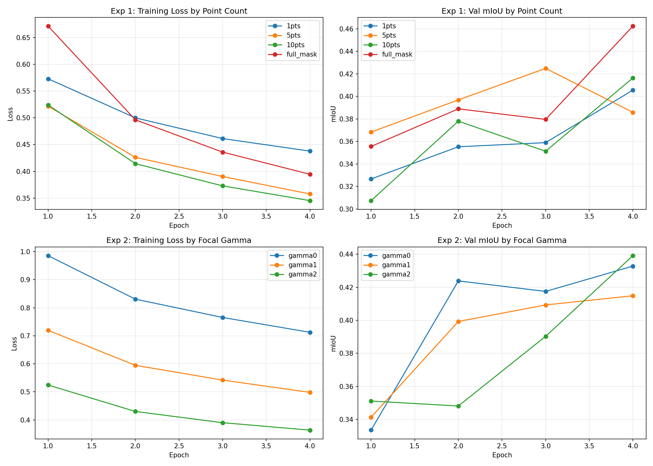
Experiment 1: How much does annotation density matter?
Question: If the network receives 1 labeled point per class instead of 10, how much segmentation quality is lost?
Setup: Four independent training runs evaluated across varying point densities: 1, 5, 10, and a dense full-mask baseline trained with standard cross-entropy.
Results:
| Condition | Epoch 1 mIoU | Final mIoU |
|---|---|---|
| 1 point | 0.327 | 0.406 |
| 5 points | 0.368 | 0.386 |
| 10 points | 0.308 | 0.416 |
| Full mask | 0.356 | 0.463 |
The dense baseline converged at 0.463 mIoU. Notably, the 10-point model reached 0.416 mIoU, sitting just 0.047 points below the upper bound despite supervising fewer than 0.1% of total pixels.
The 5-point condition finishing below the 1-point model at epoch 4 contradicts monotonic scaling assumptions. Analyzing the validation trajectories clarifies the discrepancy: the 5-point network peaked at 0.425 mIoU during epoch 3 before regressing slightly in epoch 4. At four epochs, optimization curves remain subject to single-seed variance and early optimization noise. Regardless of run-to-run variance, the macroscopic trend confirms that supervising roughly 5 total pixels per tile provides sufficient signal to resolve dense structural geometry.
Experiment 2: Does the focal gamma value matter?
Question: Is focal modulation actively driving convergence, or is partial gradient masking doing the majority of the work?
Setup: Three runs supervised at 5 points per class across fixed gamma values: 0 (standard partial cross-entropy), 1, and 2.
Results:
| Gamma | Epoch 1 mIoU | Final mIoU | Final Loss |
|---|---|---|---|
| γ = 0 | 0.334 | 0.433 | 0.712 |
| γ = 1 | 0.341 | 0.415 | 0.498 |
| γ = 2 | 0.351 | 0.439 | 0.364 |
Setting γ = 2 achieved the highest final validation score at 0.439 mIoU. However, the performance delta between full focal weighting and unweighted partial cross-entropy (γ = 0) is just 0.006 mIoU.
The raw loss values vary wildly across conditions (0.712 vs 0.364). This scale shift is a mathematical artifact of the focal modulating term compressing gradient magnitudes, not an indicator of superior convergence. Because loss magnitudes cannot be compared across differing gamma parameters, validation mIoU serves as the sole ground-truth evaluation metric.
The primary takeaway is that unweighted partial cross-entropy reaches 0.433 mIoU on its own. Isolating the gradient pool to annotated coordinates eliminates background dominance effectively, proving spatial masking is the foundational optimization mechanism, while focal weighting acts as a secondary stabilizer.
There’s a detail in my own setup that undercuts the class-imbalance story I told earlier. simulate_point_labels_single samples the same number of points for every class, so background gets exactly as many labelled points as road or water, regardless of how much of the tile each one actually covers. That means the label set the loss ever sees is already balanced 1:1:1:1:1 before focal weighting touches anything. So focal loss in this setup isn’t rebalancing class frequency. The point sampler already did that job. What’s left for gamma to do is smaller: among a handful of already-balanced labelled points, push gradient toward the ones the model is still unsure about and away from the ones it’s already confident on. Call it hard-point mining within a balanced set, not frequency correction. The 0.006 mIoU gap between γ = 0 and γ = 2 is consistent with that smaller job. If focal loss were fixing severe class imbalance the way the earlier section describes it, the gap between having it and not having it should be a lot bigger than six thousandths of a point.
Known limitations and what I would do differently
The point labels in this setup are resampled on every epoch, not fixed once per tile. simulate_point_labels_single runs inside __getitem__ and draws a fresh torch.randperm every time it’s called, so a given tile’s “five annotated points” are five different points in epoch 1 versus epoch 4. A real annotator clicks points once and that’s the permanent budget. What I built is closer to a form of data augmentation than to a genuine fixed-budget weak-supervision setup, and it likely makes the low-point-count conditions look better than a truly fixed budget would, since the model sees a rotating superset of locations across four epochs instead of one fixed sparse set. The fix is to seed the sampling once per tile, either by caching the sampled points at dataset construction or by seeding the sampler off a hash of the filename, so the simulated annotation stays fixed for the whole run the way a real one would.
The loss function computes softmax first and takes a log with an epsilon patch afterward, instead of using log_softmax. PyTorch’s own CrossEntropyLoss fuses log_softmax and nll_loss specifically to avoid this pattern, because computing probabilities first means you can end up taking the log of a number very close to zero, which gets worse under mixed precision. The epsilon hack holds up fine at fp32 with five classes, but the production fix is to compute log-probabilities directly with log_softmax and gather from there, so the masking and focal weighting sit on top of an already-stable number instead of patching an unstable one after the fact.
BatchNorm across the U-Net with a batch size of 8 gives noisy running statistics, especially with five imbalanced classes competing for those statistics inside each batch. GroupNorm is the standard swap when batch size is constrained by memory, since it normalizes within each sample instead of across the batch, and I’d make that change before scaling this to larger images where batch size only gets smaller.
I used no augmentation at all: no flips, no rotation, no color jitter. In a sparse-label regime this is probably the single biggest gap in what I built. Every tile was shown to the network exactly once per epoch in exactly one orientation, on top of the fact that most of the pixels in that tile were never labelled to begin with. Augmentation is usually optional in a fully-supervised setting. Here it’s closer to load-bearing, and leaving it out means there’s performance sitting on the table for free.
Key Takeaways
Transitioning from sequence modeling to spatial vision highlighted three core engineering realities:
Objective design dictates architectural viability. In standard language modeling, dense cross-entropy handles optimization reliably out of the box. In sparsely annotated computer vision, applying standard objectives actively destroys feature representations by backpropagating false gradients from unannotated regions.
Skip connections function as spatial memory. Bottleneck layers resolve semantic identity at highly compressed 16x16 resolutions. Skip connections preserve spatial coordinate geometry across uncompressed intermediate feature maps, allowing networks to anchor abstract class representations to exact pixel boundaries.
Training metrics and evaluation metrics measure distinct objectives. During optimization, loss is calculated over 0.038% of available pixels. At test time, validation metrics evaluate 100% of the grid. Closing that generalization gap is the fundamental challenge of weakly supervised learning.
Full code on GitHub. Dataset: LandCover.ai.
Brayan’s Blog — AI/ML Research, Engineering