Hardware Economics Blog
AI Hardware Economics
Based on the Dwarkesh Patel / Reiner Pope blackboard session — watch here
I spend the majority of my time contemplating model architecture, pretraining, reinforcement, and inference. I believed I understood the computational aspect of things fairly well. After seeing Dwarkesh Patel and Reiner Pope go over the real hardware economics of teaching and servicing LLMs for two hours at a chalkboard, I realized that this was also really intriguing and appreciated how it was all done.
This post is my attempt to write up what I learned properly. All of the analysis and numbers come from that session. I’ll go section by section.
1. The roofline model: how to think about any inference workload
Reiner opens by introducing two quantities that govern the time cost of any forward pass through a transformer:
t_compute the time to do all the matrix multiplications over the active parameters:
t_compute = (B × N_active) / FLOPs
where B is batch size, N_active is active parameters, and FLOPs is the hardware’s compute throughput.
t_mem the time to fetch weights and KV cache from memory:
t_mem = (N_total + B × len_ctx × KV_bytes_per_token) / mem_bw
The actual time for a forward pass is the maximum of these two:
T = max(t_compute, t_mem)
This is the roofline model. It will not perfectly predict the time, but it gives you the right intuitions about what is bottlenecking you and what levers you can pull.
2. Batch size, latency, and cost
Why batch size matters so much
The weight fetch in t_mem does not depend on batch size. You load the weights once regardless of how many sequences you are serving. But the compute in t_compute scales linearly with batch size. This means:
- At small batch sizes, you are memory-bandwidth-bound. Most of your time is spent loading weights that are barely used. Cost per token is high.
- As batch size grows, you amortize the weight fetch across more sequences. Cost per token drops sharply.
- At large batch sizes, you hit the compute ceiling. Cost per token flattens out at its lower bound.
At very small batch sizes, Reiner notes that the cost can be literally a thousand times worse than at an optimally batched workload.
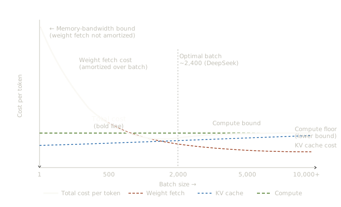 Figure 1: Cost per token vs batch size. The weight fetch cost is a hyperbola that falls as batch grows. The KV cache cost is roughly flat. The compute floor sets the lower bound. Total cost is the maximum of all three.
The optimal batch size formula
Setting t_compute = t_mem (the balance point where both resources are fully saturated) and ignoring the KV cache term:
B × N_active / FLOPs = N_total / mem_bw
Solving for B:
B ≥ (FLOPs / mem_bw) × (N_total / N_active) = 300 × (1 / sparsity)
The hardware ratio FLOPs/mem_bw is approximately 300 on modern GPUs (stable across A100, H100, B100 generations). Sparsity is the ratio of active to total parameters.
For DeepSeek V3, which activates 32 out of 256 experts (sparsity = 32/256 = 1/8):
B ≥ 300 × 8 = 2,400 sequences
That is the minimum batch size to be compute-bound rather than bandwidth-bound. The KV cache term pushes this higher as context length grows.
The train station metaphor
A useful way to think about scheduling: every ~20ms, a “train” departs carrying a batch of sequences through one forward pass, producing one new token per sequence. New requests board when they arrive. If the train is full they wait for the next one. Worst-case queuing latency is therefore 40ms one missed train plus one full forward pass.
The 20ms figure comes from the HBM drain time: memory capacity divided by memory bandwidth. On Nvidia Rubin, that is 288 GB / 20 TB/s ≈ 15ms. Running trains faster than this is physically impossible because you cannot read all the weights from HBM in less time than bandwidth allows. Running trains slower just wastes FLOPs.
3. MoE layout on GPU racks
The all-to-all problem
In a Mixture-of-Experts layer, a router decides which experts each token goes to typically a small fraction, like 6 out of 256 in DeepSeek. Each expert is a standard MLP. In expert parallelism, different experts live on different GPUs.
The communication pattern this creates is all-to-all: any GPU’s tokens may route to any other GPU’s experts, depending on the routing decision. This means every GPU needs to be able to talk to every other GPU at full bandwidth.
Within a single rack, NVLink provides exactly this: full all-to-all connectivity across all GPUs in two hops (GPU → switch → GPU). It is a perfect fit for the MoE traffic pattern.
Why crossing rack boundaries is a problem
The scale-out network connecting racks is approximately 8× slower than the NVLink scale-up network within a rack. If your MoE layer spans two racks, roughly half your tokens need to cross that slower link on every forward pass, and that becomes the bottleneck.
This makes one rack a natural boundary for an MoE layer. For DeepSeek V3 with 256 experts running on a 64-GPU Blackwell rack, that works out to 4 experts per GPU.
Nvidia has been expanding scale-up domain sizes precisely to enable larger MoE layers without rack-crossing penalties: Hopper was 8 GPUs, Blackwell is 72, Rubin will be ~500+. Google’s TPU pods have had large scale-up domains for longer, which Reiner suggests is part of why Gemini has been able to deploy high-sparsity MoE models effectively.
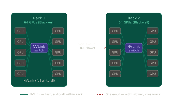 Figure 2: Within a rack, NVLink gives full all-to-all connectivity a perfect fit for MoE routing. Crossing to a second rack forces traffic through the scale-out network, which is ~8× slower. One rack is therefore a natural boundary for an MoE layer.
4. Pipeline parallelism
What it is and why you would use it
Pipeline parallelism assigns different layers of the model to different racks. Rack 1 handles layers 1–15, rack 2 handles layers 16–30, and so on. As each rack finishes its portion, it passes activations to the next rack.
The benefit is memory capacity: instead of needing the entire model on one rack, each rack only holds a fraction of the layers.
The bubble problem
Bubbles emerge because the pipeline stages are not always busy simultaneously. At the start of a batch, racks handling later layers are idle waiting for activations to arrive. At the end of a batch, early-layer racks go idle while the backward pass finishes at the end of the pipeline.
In inference, this is solved trivially you just start the next batch as soon as the first batch passes through the first stage. There is no real cost.
In training, it is harder. You cannot just overlap batches, because you need to consolidate gradients and update the weights before processing the next batch. Various techniques (zero bubble, 1F1B interleaving) try to mitigate this, but it remains a real efficiency cost.
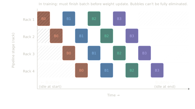 Figure 3: Pipeline parallelism during training. Batches flow diagonally through pipeline stages. The gray hatched regions at the start and end of each batch are the “bubble” idle time where racks are waiting. This cannot be eliminated in training without techniques like zero bubble or 1F1B interleaving.
Why pipelining does not help with KV cache
Pipeline parallelism divides model weights by P (number of stages) per device. You might expect it to also divide the KV cache by P. It does not.
To keep P pipeline stages busy simultaneously, you need P micro-batches in flight at once. The number of concurrent sequences scales with P. KV cache footprint per GPU therefore stays constant regardless of how many pipeline stages you add. The math exactly cancels.
Given that KV cache dominates memory at long context lengths, this severely limits the practical value of pipelining for inference.
Why Ilya said “pipelining is not wise”
Beyond the efficiency costs, pipeline parallelism imposes hard architectural constraints. Architectures where attention in one block attends to residuals from previous blocks (like Kimi) become very difficult to implement when those residuals live on different racks. Interleaving sliding-window and global attention layers can cause load imbalance across stages. All of this slows down research iteration, which Reiner describes as the bigger sin.
5. The 6ND formula and compute cost breakdown
Where the 6 comes from
The 6ND formula for pretraining FLOPs is one of the most referenced numbers in ML, and almost nobody explains where it comes from:
- 2ND: forward pass 2 FLOPs per parameter per token (one multiply, one add)
- 4ND: backward pass 2× the forward pass, because you compute gradients with respect to both input matrices
- Total: 6ND
Total compute across pretraining, RL, and inference
The full cost equation:
C_total = C_pretrain + C_RL + C_inference

C_pretrain  = 6 × N_active × D_pretrain
C_RL        = (2 to 6) × N_active × D_RL × inefficiency
C_inference = 2 × N_active × D_inference × inefficiency
RL is 2–6× because: 2 if you only do a forward pass on rollouts and do not train on all of them, up to 6 if you run full forward and backward on every generation. The inefficiency term (~⅓) reflects that decode runs at much lower MFU than prefill.
Inference is 2× (forward only), also with a decode efficiency penalty.
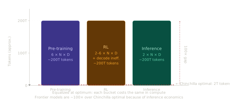 Figure 4: At the optimum, pretraining, RL, and inference costs are roughly equal. Each bucket corresponds to ~200T tokens for a frontier model. That is ~100× the Chinchilla-optimal token count.
The equalization heuristic
Reiner’s key heuristic: if pretraining, RL, and inference costs trade off (more pretraining means less RL/inference needed for the same quality), then the optimum is approximately where all three costs are equal. Setting them equal and solving:
D_pretrain ≈ 1.5 × D_RL ≈ D_inference
So the number of pretraining tokens and the number of inference tokens served should be in roughly the same ballpark.
How over-trained are frontier models?
Grounding this with real numbers:
- A frontier model serving 50M tokens/second globally for 2 months accumulates approximately 200T inference tokens
- Therefore D_pretrain should also be around 200T tokens
- Chinchilla optimal for a model with 100B active parameters is 20 × N_active = 2T tokens
- Ratio: 200T / 2T = 100×
Frontier models are approximately 100× over Chinchilla-optimal, almost entirely because of inference economics and RL, not because pretraining is inefficient in isolation. The Chinchilla rule was derived to minimise training compute. It says nothing about inference.
6. What API pricing tells you about hardware
The Gemini 200K crossover
Gemini charges ~50% more for tokens above 200K context. Here is what that tells you:
- Below 200K: compute-bound. Marginal cost per token is flat as context grows.
- Above 200K: memory-bandwidth-bound. KV cache fetch time overtakes compute time, and marginal cost rises linearly with context length.
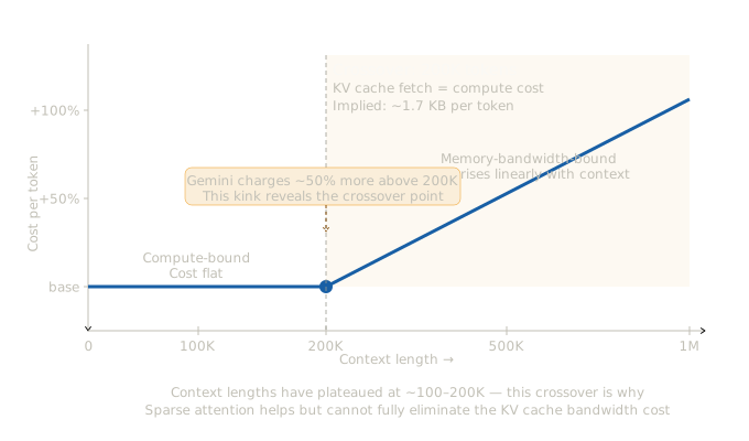 Figure 5: Cost per token is flat up to ~200K tokens (compute-bound), then rises linearly (memory-bandwidth-bound). The kink in Gemini’s pricing directly reveals this crossover point. Above 200K, you are paying for KV cache bandwidth, not compute.
The crossover is where t_compute = t_KV_fetch. Setting them equal:
B × N_active / FLOPs = B × len_ctx × bytes_per_token / mem_bw
Solving for bytes per token:
bytes_per_token = (mem_bw / FLOPs) × (N_active / len_ctx)
                = (1/300) × (100B / 200K)
                ≈ 1.7 KB per token
From a single pricing datapoint, you can back out that Gemini’s KV cache is approximately 1.7 KB per token at that scale. Plausible with 8 KV heads at d_head = 128 across multiple layers, or via sparse attention variants.
Why output tokens cost more than input tokens
Output tokens (decode) are typically 3–5× more expensive than input tokens (prefill). The reason:
- During prefill, you process the whole sequence in parallel. The weight fetch is amortized across many tokens of compute. MFU is high.
- During decode, you load all the weights just to produce one new token. The weight fetch cost is not amortized at all. MFU drops to roughly ⅕ of prefill.
This is why Claude and Codex offer “Fast Mode” at 6× the price for 2.5× the speed you are paying for a smaller, less amortized batch.
Cache pricing and memory tiers
Cached tokens (cache hits) are ~10× cheaper than fresh input tokens because loading KVs from memory is much cheaper than recomputing them from token IDs. API providers offer different cache durations (e.g. 5 minutes vs 1 hour) at different prices, which you can use to infer which memory tier is being used:
The drain time of a memory tier capacity divided by bandwidth determines how long it makes sense to hold something there before it becomes cheaper to evict and recompute. HBM drain time is ~20ms (too short for caching). DDR is on the order of seconds. Flash is on the order of minutes. Spinning disk is on the order of hours. A 5-minute cache tier is consistent with flash; a 1-hour tier is consistent with spinning disk.
The long context wall
The fundamental barrier to very long context (100M+ tokens) is memory bandwidth, not compute. The KV cache fetch time scales linearly with context length, and HBM bandwidth is not improving fast enough to keep pace. Sparse attention helps it can give you a square root improvement but not infinitely, because going too sparse hurts quality.
Reiner notes that context lengths have been hovering around 100–200K for the past couple of years. That plateau is not a coincidence. It reflects where the memory bandwidth cost becomes prohibitive. There is no clean path to solving this on current hardware.
7. Convergent evolution: neural networks and cryptography
The session closes with a fascinating detour into the structural similarities between neural networks and cryptographic ciphers.
Both need every output to depend on every input in complicated, hard-to-invert ways. Cryptographic protocols achieve this through mixing and scrambling across many rounds. Neural networks do it through layers of matrix multiplications and nonlinearities. The architectures have converged toward similar high-level structures independently.
The key difference: cryptographic protocols are trying to destroy structure take something with regularity and make it indistinguishable from random. Neural networks are trying to extract structure take something that looks random and find the underlying pattern. Same mechanism, opposite goal.
One direct import from cryptography into deep learning is the Feistel network, introduced in the 2017 RevNets paper. A Feistel construction makes any function invertible by maintaining two streams and alternating which one gets transformed:
Given inputs (x, y):
output_x = x
output_y = y + f(x)

To invert: recover x directly, then recover y = output_y - f(output_x)
Applied to a transformer layer, this makes the entire network invertible. The benefit for training: because you can regenerate any activation by running the network forward from the input, you do not need to store intermediate activations during the forward pass. You recompute them on demand during the backward pass, trading compute for memory the inverse of what the KV cache does.
Final thought
The most productive reframe from this session: a transformer is not just a mathematical object, it is a physical system running on hardware with bandwidth constraints, capacity limits, and thermal envelopes. The architecture choices, the sparsity decisions, the context length limits, the API pricing tiers they all follow from the physics of moving bytes around. Once you see it that way, a lot of things that seemed arbitrary start to look inevitable.
The video is here: https://www.youtube.com/watch?v=xmkSf5IS-zw highly recommend watching with a pen and paper.