<?xml version="1.0" encoding="utf-8"?><feed xmlns="http://www.w3.org/2005/Atom" ><generator uri="https://jekyllrb.com/" version="3.10.0">Jekyll</generator><link href="https://brayanbrayan.github.io/feed.xml" rel="self" type="application/atom+xml" /><link href="https://brayanbrayan.github.io/" rel="alternate" type="text/html" /><updated>2026-04-02T12:48:09+00:00</updated><id>https://brayanbrayan.github.io/feed.xml</id><title type="html">Brayan’s Blog</title><subtitle>AI/ML Research, Engineering</subtitle><author><name>Brayan</name></author><entry><title type="html">RLHF from Scratch: A Complete Alignment Study</title><link href="https://brayanbrayan.github.io/2026/04/02/rlhf-post-blog.html" rel="alternate" type="text/html" title="RLHF from Scratch: A Complete Alignment Study" /><published>2026-04-02T00:00:00+00:00</published><updated>2026-04-02T00:00:00+00:00</updated><id>https://brayanbrayan.github.io/2026/04/02/rlhf-post-blog</id><content type="html" xml:base="https://brayanbrayan.github.io/2026/04/02/rlhf-post-blog.html"><![CDATA[<p><em>Personal project · 2026 · PyTorch · tatsu-lab/alpaca · 1M parameter model</em></p>

<hr />

<h2 id="table-of-contents">Table of Contents</h2>

<ol>
  <li><a href="#1-overview">Overview</a></li>
  <li><a href="#2-the-four-algorithms">The four algorithms</a>
    <ul>
      <li><a href="#21-supervised-fine-tuning-sft--the-baseline">2.1 SFT — the baseline</a></li>
      <li><a href="#22-ppo--proximal-policy-optimisation">2.2 PPO</a></li>
      <li><a href="#23-grpo--group-relative-policy-optimisation">2.3 GRPO</a></li>
      <li><a href="#24-dpo--direct-preference-optimisation">2.4 DPO</a></li>
    </ul>
  </li>
  <li><a href="#3-phase-1--baseline-evaluation">Phase 1 — Baseline evaluation</a></li>
  <li><a href="#4-phase-5--hyperparameter-tuning">Phase 5 — Hyperparameter tuning</a></li>
  <li><a href="#5-dpo-training-dynamics-phase-1-vs-phase-5">DPO training dynamics</a></li>
  <li><a href="#6-grpo-group-collapse-phase-1-vs-phase-5">GRPO group collapse</a></li>
  <li><a href="#7-phase-5--results">Phase 5 results</a></li>
  <li><a href="#8-per-prompt-delta-analysis">Per-prompt delta analysis</a></li>
  <li><a href="#9-the-ranking-reversal">The ranking reversal</a></li>
  <li><a href="#10-conclusion">Conclusion</a></li>
</ol>

<hr />

<h2 id="1-overview">1. Overview</h2>

<p>This is the final report of a ten part project implementing reinforcement learning from human feedback (RLHF) entirely from scratch in PyTorch. Every component the tokenizer, the language model, the reward model, and all three post-SFT alignment algorithms were built from first principles without relying on pretrained weights or alignment libraries.</p>

<p>The project runs two evaluation phases. <strong>Phase 1</strong> establishes baselines by running SFT, PPO, GRPO, and DPO checkpoints through a fixed evaluation suite of 16 prompts scored by a trained reward model. <strong>Phase 5</strong> reruns all four algorithms with targeted hyperparameter changes, motivated by the specific failure modes identified in Phase 1. The result is a complete before-and-after picture of what each algorithm does, what breaks it, and what fixes it.
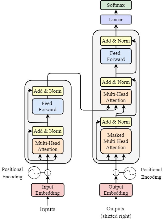
</p>

<h3 id="architecture">Architecture</h3>

<p>All four models share the same architecture throughout:</p>

<table>
  <thead>
    <tr>
      <th>Component</th>
      <th>Value</th>
    </tr>
  </thead>
  <tbody>
    <tr>
      <td>Layers</td>
      <td>2</td>
    </tr>
    <tr>
      <td>Attention heads</td>
      <td>2</td>
    </tr>
    <tr>
      <td>Embedding dim</td>
      <td>128</td>
    </tr>
    <tr>
      <td>Parameters</td>
      <td>~1M</td>
    </tr>
    <tr>
      <td>Tokenizer</td>
      <td>BPE, 8,000 vocab</td>
    </tr>
    <tr>
      <td>Block size</td>
      <td>256 tokens</td>
    </tr>
    <tr>
      <td>Reward model</td>
      <td>4-layer, 256-dim bidirectional transformer</td>
    </tr>
  </tbody>
</table>

<blockquote>
  <p><strong>Evaluation protocol:</strong> All scores come from the same reward model scoring the same 16 prompts from <code class="language-plaintext highlighter-rouge">tatsu-lab/alpaca</code> via <code class="language-plaintext highlighter-rouge">sample_prompts()</code>. Phase 1 generation uses <code class="language-plaintext highlighter-rouge">temperature=0.7, top_k=50, max_new_tokens=64</code>. Phase 5 uses <code class="language-plaintext highlighter-rouge">temperature=0.3, top_k=20, max_new_tokens=96</code>. The same protocol for all methods makes scores directly comparable within each phase.</p>
</blockquote>

<hr />

<h2 id="2-the-four-algorithms">2. The four algorithms</h2>

<h3 id="21-supervised-fine-tuning-sft--the-baseline">2.1 Supervised Fine-Tuning (SFT) — the baseline</h3>

<p>SFT is not an alignment algorithm it is the starting point for all three. The SFT model is fine-tuned on <code class="language-plaintext highlighter-rouge">tatsu-lab/alpaca</code> using standard cross-entropy loss over the response tokens only, learning to imitate the distribution of human-written instruction responses.</p>

<p>The SFT checkpoint serves two roles: it is both the evaluation baseline that all post-SFT methods must beat, and the initialisation point from which PPO, GRPO, and DPO all start.</p>

<hr />

<h3 id="22-ppo--proximal-policy-optimisation">2.2 PPO — Proximal Policy Optimisation</h3>

<p>PPO frames alignment as a reinforcement learning problem. The policy generates rollouts (responses), the reward model scores them, and the policy is updated to maximise reward subject to a KL constraint preventing too much drift from the reference model.</p>

<p><strong>The KL-constrained RL objective:</strong></p>

<p><img src="/images/rlhfblogimages/math_ppo_objective.png" alt="KL-constrained RL objective" />
<!-- INSERT: math_ppo_objective.png --></p>

<p><strong>The clipped surrogate loss:
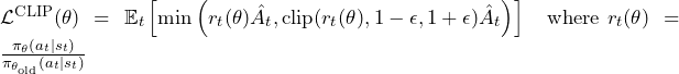
</strong></p>

<p><img src="/images/rlhfblogimages/math_ppo_loss.png" alt="The clipped surrogate loss" />
<!-- INSERT: math_ppo_loss.png --></p>

<p>Where <code class="language-plaintext highlighter-rouge">r_t(θ) = π_θ(aₜ|sₜ) / π_old(aₜ|sₜ)</code> is the probability ratio and <code class="language-plaintext highlighter-rouge">Â_t</code> is the advantage estimated by the value head using GAE.</p>

<p><strong>The shaped reward used at each token position:</strong></p>

<p><img src="/images/rlhfblogimages/math_ppo_shaped_reward.png" alt="The shaped reward used at each token position" />
<!-- INSERT: math_ppo_shaped_reward.png --></p>

<div class="language-python highlighter-rouge"><div class="highlight"><pre class="highlight"><code><span class="n">shaped_reward</span><span class="p">[</span><span class="n">t</span><span class="p">]</span> <span class="o">=</span> <span class="n">r_scalar</span> <span class="o">-</span> <span class="n">kl_coef</span> <span class="o">*</span> <span class="p">(</span><span class="n">log_pi_theta</span><span class="p">[</span><span class="n">t</span><span class="p">]</span> <span class="o">-</span> <span class="n">log_pi_ref</span><span class="p">[</span><span class="n">t</span><span class="p">])</span>

<span class="c1"># Phase 1: kl_coef = 0.01
# Phase 5: kl_coef = 0.1
</span></code></pre></div></div>

<hr />

<h3 id="23-grpo--group-relative-policy-optimisation">2.3 GRPO — Group Relative Policy Optimisation</h3>

<p>
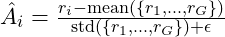
GRPO eliminates the value function entirely. Instead of estimating a baseline from a critic, it generates a group of <code class="language-plaintext highlighter-rouge">k</code> responses to the same prompt and uses the group statistics as the baseline. The advantage for each response is its normalised position within the group.</p>

<p><strong>Group-relative advantage:</strong></p>

<p><img src="/images/rlhfblogimages/math_grpo_advantage.png" alt="Group-relative advantage" />
<!-- INSERT: math_grpo_advantage.png --></p>

<p><strong>The GRPO loss:</strong></p>

<p><img src="/images/rlhfblogimages/math_grpo_loss.png" alt="The GRPO loss" />
<!-- INSERT: math_grpo_loss.png --></p>

<p>The critical vulnerability: when all <code class="language-plaintext highlighter-rouge">k</code> responses are near-identical, <code class="language-plaintext highlighter-rouge">std(r) → 0</code> and all advantages <code class="language-plaintext highlighter-rouge">→ 0</code>. No gradient flows. This is <strong>group collapse</strong>, and it is GRPO’s primary failure mode at small model scale.</p>

<div class="language-python highlighter-rouge"><div class="highlight"><pre class="highlight"><code><span class="n">rewards</span>    <span class="o">=</span> <span class="n">torch</span><span class="p">.</span><span class="n">tensor</span><span class="p">([</span><span class="n">rm</span><span class="p">(</span><span class="n">resp_i</span><span class="p">)</span> <span class="k">for</span> <span class="n">i</span> <span class="ow">in</span> <span class="nb">range</span><span class="p">(</span><span class="n">k</span><span class="p">)])</span>
<span class="n">mean_r</span>     <span class="o">=</span> <span class="n">rewards</span><span class="p">.</span><span class="n">mean</span><span class="p">()</span>
<span class="n">std_r</span>      <span class="o">=</span> <span class="n">rewards</span><span class="p">.</span><span class="n">std</span><span class="p">().</span><span class="n">clamp_min</span><span class="p">(</span><span class="mf">1e-6</span><span class="p">)</span>   <span class="c1"># prevents div-by-zero
</span><span class="n">advantages</span> <span class="o">=</span> <span class="p">(</span><span class="n">rewards</span> <span class="o">-</span> <span class="n">mean_r</span><span class="p">)</span> <span class="o">/</span> <span class="n">std_r</span>      <span class="c1"># (k,) — zero if all same
</span>
<span class="c1"># Phase 1: k=4, gen_temp=0.8
# Phase 5: k=8, gen_temp=1.0
</span></code></pre></div></div>

<hr />

<h3 id="24-dpo--direct-preference-optimisation">2.4 DPO — Direct Preference Optimisation</h3>

<p>DPO eliminates both the explicit reward model and the RL loop from training. Instead, it reparameterises the optimal policy in terms of log-ratios between the policy and reference, then derives a loss directly over preference pairs (chosen, rejected).</p>

<p>
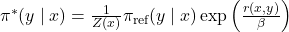
The key insight from Rafailov et al. (NeurIPS 2023) is that the optimal policy under the KL-constrained reward objective satisfies:</p>

<p><strong>Optimal policy form:</strong></p>

<p><img src="/images/rlhfblogimages/math_dpo_optimal_policy.png" alt="Optimal policy form" />
<!-- INSERT: math_dpo_optimal_policy.png --></p>

<p>Rearranging to express reward in terms of the policy:</p>

<p><strong>Reward reparameterisation:</strong></p>

<p><img src="/images/rlhfblogimages/math_dpo_reward_reparam.png" alt="Reward reparameterisation" />
<!-- INSERT: math_dpo_reward_reparam.png --></p>

<p>
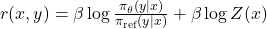
Substituting into the Bradley-Terry preference model causes <code class="language-plaintext highlighter-rouge">Z(x)</code> to cancel, yielding the DPO loss:</p>

<p><strong>The DPO loss:</strong></p>

<p><img src="/images/rlhfblogimages/math_dpo_loss.png" alt="The DPO loss" />
<!-- INSERT: math_dpo_loss.png --></p>

<blockquote>
  <p>The reward model does not appear anywhere in the DPO training loop. It is used only for post-hoc evaluation in <code class="language-plaintext highlighter-rouge">dpo_logger.py</code> and <code class="language-plaintext highlighter-rouge">eval_dpo.py</code>. This is the key architectural distinction from PPO and GRPO.</p>
</blockquote>

<p><strong>The <code class="language-plaintext highlighter-rouge">get_logps</code> function — the shift logic that must be correct:</strong></p>

<div class="language-python highlighter-rouge"><div class="highlight"><pre class="highlight"><code><span class="k">def</span> <span class="nf">get_logps</span><span class="p">(</span><span class="n">model</span><span class="p">,</span> <span class="n">input_ids</span><span class="p">,</span> <span class="n">response_mask</span><span class="p">):</span>
    <span class="n">logits</span><span class="p">,</span> <span class="n">_</span><span class="p">,</span> <span class="n">_</span> <span class="o">=</span> <span class="n">model</span><span class="p">.</span><span class="n">lm</span><span class="p">(</span><span class="n">input_ids</span><span class="p">,</span> <span class="bp">None</span><span class="p">)</span>     <span class="c1"># (B, T, V)
</span>    <span class="n">shift_logits</span> <span class="o">=</span> <span class="n">logits</span><span class="p">[:,</span> <span class="p">:</span><span class="o">-</span><span class="mi">1</span><span class="p">,</span> <span class="p">:]</span>              <span class="c1"># predict positions 1..T
</span>    <span class="n">shift_labels</span> <span class="o">=</span> <span class="n">input_ids</span><span class="p">[:,</span> <span class="mi">1</span><span class="p">:]</span>               <span class="c1"># actual tokens 1..T
</span>    <span class="n">shift_mask</span>   <span class="o">=</span> <span class="n">response_mask</span><span class="p">[:,</span> <span class="mi">1</span><span class="p">:]</span>           <span class="c1"># only response positions
</span>    <span class="n">log_probs</span>    <span class="o">=</span> <span class="n">torch</span><span class="p">.</span><span class="n">log_softmax</span><span class="p">(</span><span class="n">shift_logits</span><span class="p">,</span> <span class="n">dim</span><span class="o">=-</span><span class="mi">1</span><span class="p">)</span>
    <span class="n">token_logps</span>  <span class="o">=</span> <span class="n">log_probs</span><span class="p">.</span><span class="n">gather</span><span class="p">(</span><span class="o">-</span><span class="mi">1</span><span class="p">,</span> <span class="n">shift_labels</span><span class="p">.</span><span class="n">unsqueeze</span><span class="p">(</span><span class="o">-</span><span class="mi">1</span><span class="p">)).</span><span class="n">squeeze</span><span class="p">(</span><span class="o">-</span><span class="mi">1</span><span class="p">)</span>
    <span class="k">return</span> <span class="p">(</span><span class="n">token_logps</span> <span class="o">*</span> <span class="n">shift_mask</span><span class="p">.</span><span class="nb">float</span><span class="p">()).</span><span class="nb">sum</span><span class="p">(</span><span class="n">dim</span><span class="o">=-</span><span class="mi">1</span><span class="p">)</span>  <span class="c1"># (B,)
</span>
<span class="c1"># Phase 1: beta=0.1
# Phase 5: beta=0.3
</span></code></pre></div></div>

<hr />

<h2 id="3-phase-1--baseline-evaluation">3. Phase 1 — Baseline evaluation</h2>

<p>All four checkpoints were evaluated on the same 16 prompts with the same reward model at <code class="language-plaintext highlighter-rouge">temperature=0.7, top_k=50</code>.</p>

<h3 id="per-prompt-results">Per-prompt results</h3>

<p><img src="/images/rlhfblogimages/fig1_phase1_per_prompt.png" alt="Per-prompt results" />
<!-- INSERT: fig1_phase1_per_prompt.png --></p>

<p><em>
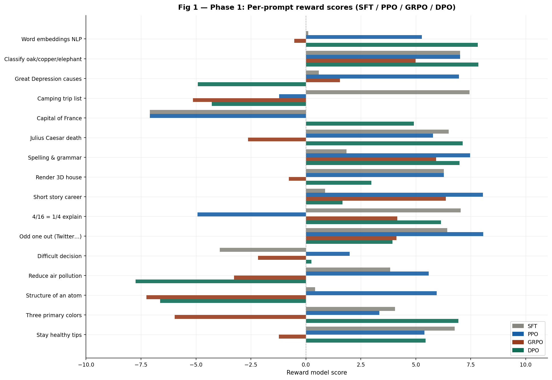
Fig 1 — Phase 1 per-prompt reward scores across all four methods.</em></p>

<h3 id="average-reward-by-algorithm">Average reward by algorithm</h3>

<p><img src="/images/rlhfblogimages/fig2_phase1_averages.png" alt="Average reward by algorithm" />
<!-- INSERT: fig2_phase1_averages.png --></p>

<p><em>
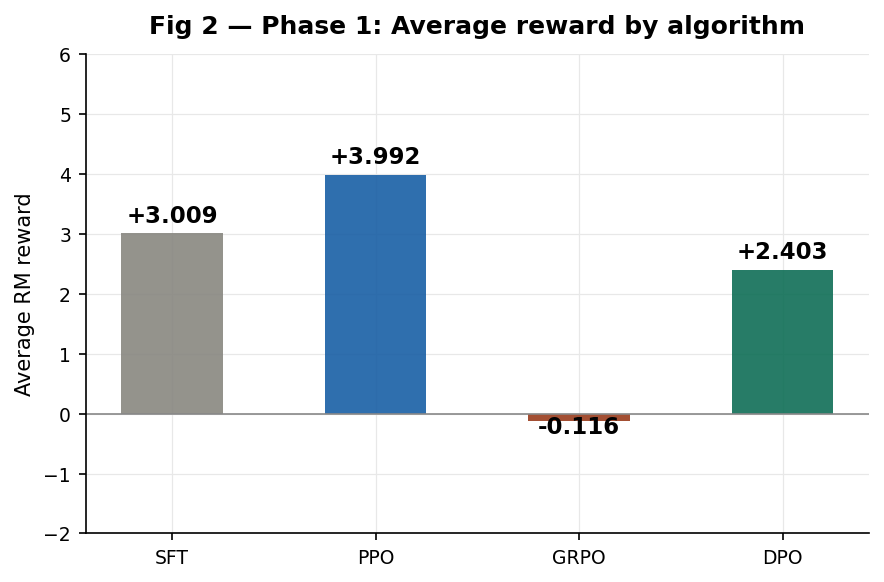
Fig 2 Phase 1 average reward. PPO wins at +3.99. GRPO is the only method below the SFT baseline.</em></p>

<h3 id="summary-table">Summary table</h3>

<table>
  <thead>
    <tr>
      <th>Prompt</th>
      <th>SFT</th>
      <th>PPO</th>
      <th>GRPO</th>
      <th>DPO</th>
    </tr>
  </thead>
  <tbody>
    <tr>
      <td>Stay healthy tips</td>
      <td>+6.77</td>
      <td>+5.39</td>
      <td>-1.23</td>
      <td>+5.44</td>
    </tr>
    <tr>
      <td>Three primary colors</td>
      <td>+4.05</td>
      <td>+3.34</td>
      <td><strong>-5.97</strong></td>
      <td>+6.93</td>
    </tr>
    <tr>
      <td>Structure of an atom</td>
      <td>+0.42</td>
      <td>+5.95</td>
      <td><strong>-7.25</strong></td>
      <td>-6.63</td>
    </tr>
    <tr>
      <td>Reduce air pollution</td>
      <td>+3.83</td>
      <td>+5.58</td>
      <td>-3.27</td>
      <td><strong>-7.75</strong></td>
    </tr>
    <tr>
      <td>Difficult decision</td>
      <td>-3.92</td>
      <td>+1.99</td>
      <td>-2.18</td>
      <td>+0.25</td>
    </tr>
    <tr>
      <td>Odd one out (Twitter…)</td>
      <td>+6.43</td>
      <td><strong>+8.07</strong></td>
      <td>+4.12</td>
      <td>+3.94</td>
    </tr>
    <tr>
      <td>4/16 = 1/4 explain</td>
      <td>+7.04</td>
      <td>-4.93</td>
      <td>+4.16</td>
      <td>+6.14</td>
    </tr>
    <tr>
      <td>Short story career</td>
      <td>+0.87</td>
      <td><strong>+8.05</strong></td>
      <td>+6.37</td>
      <td>+1.67</td>
    </tr>
    <tr>
      <td>Render 3D house</td>
      <td>+6.27</td>
      <td>+6.27</td>
      <td>-0.77</td>
      <td>+2.97</td>
    </tr>
    <tr>
      <td>Spelling &amp; grammar</td>
      <td>+1.85</td>
      <td>+7.47</td>
      <td>+5.92</td>
      <td>+6.99</td>
    </tr>
    <tr>
      <td>Julius Caesar death</td>
      <td>+6.49</td>
      <td>+5.78</td>
      <td>-2.63</td>
      <td><strong>+7.13</strong></td>
    </tr>
    <tr>
      <td>Capital of France</td>
      <td>-7.10</td>
      <td>-7.10</td>
      <td>+0.01</td>
      <td>+4.91</td>
    </tr>
    <tr>
      <td>Camping trip list</td>
      <td><strong>+7.44</strong></td>
      <td>-1.21</td>
      <td>-5.14</td>
      <td>-4.28</td>
    </tr>
    <tr>
      <td>Great Depression causes</td>
      <td>+0.59</td>
      <td>+6.96</td>
      <td>+1.55</td>
      <td>-4.91</td>
    </tr>
    <tr>
      <td>Classify oak/copper/eleph</td>
      <td>+7.01</td>
      <td>+7.01</td>
      <td>+4.99</td>
      <td><strong>+7.84</strong></td>
    </tr>
    <tr>
      <td>Word embeddings NLP</td>
      <td>+0.11</td>
      <td>+5.27</td>
      <td>-0.53</td>
      <td><strong>+7.82</strong></td>
    </tr>
    <tr>
      <td><strong>AVERAGE</strong></td>
      <td><strong>+3.009</strong></td>
      <td><strong>+3.992</strong></td>
      <td><strong>-0.116</strong></td>
      <td><strong>+2.403</strong></td>
    </tr>
  </tbody>
</table>

<p><em>Bold = highest score in row.</em></p>

<h3 id="phase-1-findings">Phase 1 findings</h3>

<p><strong>PPO</strong> wins Phase 1 at +3.99 but fails on prompts where SFT was already strong. The camping list drops from +7.44 to -1.21. The capital of France scores identically to SFT at -7.10 the policy learned nothing on that prompt.</p>

<p><strong>GRPO</strong> is the only method to regress below SFT (-0.12 average). “What are the three primary colors?” yields -5.97 because all four generated samples collapsed to “Theal” with group std ≈ 0. No gradient flowed on this prompt type.</p>

<p><strong>DPO</strong> has the highest variance of any method +7.82 on word embeddings and -7.75 on air pollution in the same evaluation run. Reward margin explosion (reaching 599 by step 150) caused catastrophic forgetting on specific prompt types.</p>

<blockquote>
  <p><strong>On reward model reliability:</strong> The capital of France is Paris scores -7.10 under both SFT and PPO. Meanwhile incoherent DPO output scores +4.91. The reward model penalises short, definitive answers regardless of correctness. All Phase 1 rankings must be read with this caveat in mind.</p>
</blockquote>

<hr />

<h2 id="4-phase-5--hyperparameter-tuning">4. Phase 5 — Hyperparameter tuning</h2>

<p>Each algorithm’s Phase 1 failure mode was diagnosed and a targeted multi-parameter tweak was applied. One retrain per algorithm, all changes applied simultaneously, evaluated with improved sampling (<code class="language-plaintext highlighter-rouge">temperature=0.3, top_k=20</code>).</p>

<h3 id="41-sft--sampling-only-no-retraining">4.1 SFT — sampling only, no retraining</h3>

<table>
  <thead>
    <tr>
      <th>Parameter</th>
      <th>Phase 1 → Phase 5</th>
      <th>Rationale</th>
    </tr>
  </thead>
  <tbody>
    <tr>
      <td>temperature</td>
      <td>0.7 → <strong>0.3</strong></td>
      <td>Forces model to commit to highest-probability tokens</td>
    </tr>
    <tr>
      <td>top_k</td>
      <td>50 → <strong>20</strong></td>
      <td>Tighter nucleus sampling, higher output consistency</td>
    </tr>
    <tr>
      <td>max_new_tokens</td>
      <td>64 → <strong>96</strong></td>
      <td>More complete responses for the RM to score</td>
    </tr>
  </tbody>
</table>

<h3 id="42-ppo--stronger-kl-constraint">4.2 PPO — stronger KL constraint</h3>

<p><em>Phase 1 diagnosis: kl_coef=0.01 was too weak to prevent forgetting of SFT-strong prompts.</em></p>

<table>
  <thead>
    <tr>
      <th>Parameter</th>
      <th>Phase 1 → Phase 5</th>
      <th>Rationale</th>
    </tr>
  </thead>
  <tbody>
    <tr>
      <td>kl_coef</td>
      <td>0.01 → <strong>0.1</strong></td>
      <td>10× stronger KL anchor to reference</td>
    </tr>
    <tr>
      <td>learning rate</td>
      <td>1e-5 → <strong>5e-6</strong></td>
      <td>Slower updates, less aggressive policy drift</td>
    </tr>
    <tr>
      <td>resp_len</td>
      <td>64 → <strong>96</strong></td>
      <td>Longer rollouts give RM more signal</td>
    </tr>
    <tr>
      <td>eval temp / top_k</td>
      <td>0.7/50 → <strong>0.3/20</strong></td>
      <td>Consistent with other methods</td>
    </tr>
  </tbody>
</table>

<h3 id="43-grpo--larger-group-higher-diversity">4.3 GRPO — larger group, higher diversity</h3>

<p><em>Phase 1 diagnosis: group collapse. With k=4 on a low-entropy model, many steps had std ≈ 0.</em></p>

<table>
  <thead>
    <tr>
      <th>Parameter</th>
      <th>Phase 1 → Phase 5</th>
      <th>Rationale</th>
    </tr>
  </thead>
  <tbody>
    <tr>
      <td>group_size k</td>
      <td>4 → <strong>8</strong></td>
      <td>More samples per group, lower collapse probability</td>
    </tr>
    <tr>
      <td>gen_temperature</td>
      <td>0.8 → <strong>1.0</strong></td>
      <td>Higher entropy during rollout keeps group std positive</td>
    </tr>
    <tr>
      <td>learning rate</td>
      <td>1e-5 → <strong>5e-6</strong></td>
      <td>Stabilises noisy diverse batches</td>
    </tr>
  </tbody>
</table>

<h3 id="44-dpo--stronger-β-slower-learning-rate">4.4 DPO — stronger β, slower learning rate</h3>

<p><em>Phase 1 diagnosis: reward margin explosion. With β=0.1, the margin reached 599 by step 150.</em></p>

<p>
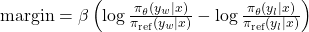
β controls how strongly large margins are penalised in the loss:</p>

<p><strong>DPO reward margin:</strong></p>

<p><img src="/images/rlhfblogimages/math_dpo_margin.png" alt="DPO reward margin" />
<!-- INSERT: math_dpo_margin.png --></p>

<table>
  <thead>
    <tr>
      <th>Parameter</th>
      <th>Phase 1 → Phase 5</th>
      <th>Rationale</th>
    </tr>
  </thead>
  <tbody>
    <tr>
      <td>beta β</td>
      <td>0.1 → <strong>0.3</strong></td>
      <td>3× stronger implicit KL, slows margin explosion</td>
    </tr>
    <tr>
      <td>learning rate</td>
      <td>1e-5 → <strong>5e-6</strong></td>
      <td>Combined with stronger β prevents catastrophic drift</td>
    </tr>
    <tr>
      <td>rej_temperature</td>
      <td>0.9 → <strong>1.1</strong></td>
      <td>More diverse rejected responses, cleaner preference signal</td>
    </tr>
  </tbody>
</table>

<hr />

<h2 id="5-dpo-training-dynamics-phase-1-vs-phase-5">5. DPO training dynamics: Phase 1 vs Phase 5</h2>

<p>The DPO training logs provide the clearest picture of what the β change achieved.</p>

<p><img src="/images/rlhfblogimages/fig3_dpo_training_dynamics.png" alt=" DPO training dynamics" />
<!-- INSERT: fig3_dpo_training_dynamics.png --></p>

<p><em>
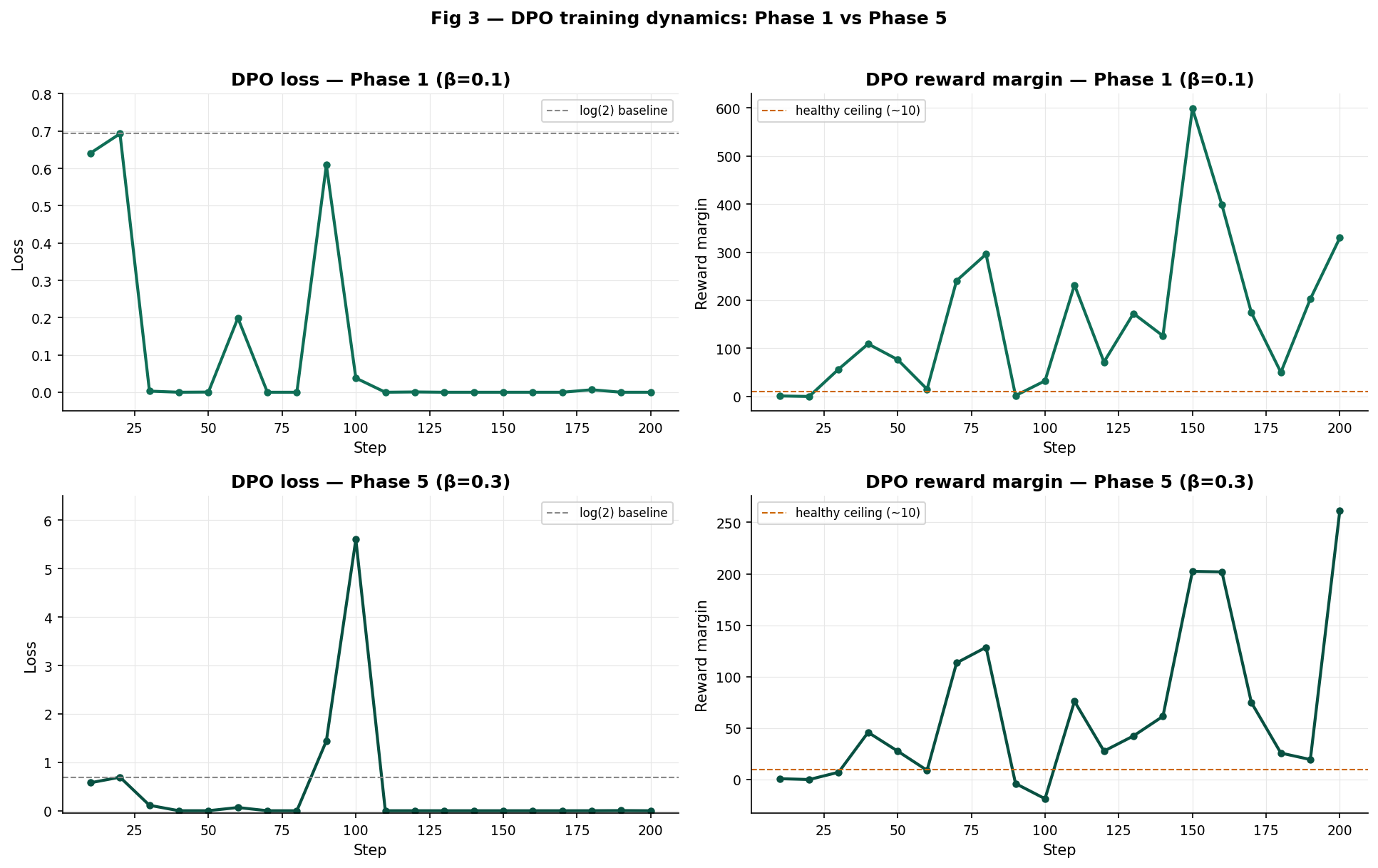
Fig 3 DPO training dynamics. Top row: Phase 1 (β=0.1). Bottom row: Phase 5 (β=0.3). Left: loss. Right: reward margin.</em></p>

<p><strong>Phase 1 (β=0.1):</strong> Loss collapses to ~0 by step 30 and stays there. The reward margin grows monotonically, reaching 599 at step 150. The model is overfitting each pair to zero loss with no recovery.</p>

<p><strong>Phase 5 (β=0.3):</strong> The loss shows genuine variation several steps near zero, but recoveries at steps 90 (1.44) and 100 (5.60). The margin peaks at 261 rather than 599, and shows negative values at steps 90 and 100, indicating the model occasionally prefers the rejected response a healthier training signal that triggers correction.</p>

<p>The negative margins in Phase 5 are not failures. They are the loss function doing its job when margin is negative, loss is high, a strong gradient fires, and the policy corrects. With β=0.1, loss reached zero so fast that these corrections never registered.</p>

<hr />

<h2 id="6-grpo-group-collapse-phase-1-vs-phase-5">6. GRPO group collapse: Phase 1 vs Phase 5</h2>

<p>The group standard deviation is the critical GRPO diagnostic. When <code class="language-plaintext highlighter-rouge">std → 0</code>, advantages <code class="language-plaintext highlighter-rouge">→ 0</code>, and no gradient flows.</p>

<p><img src="/images/rlhfblogimages/fig4_grpo_group_std.png" alt="GRPO group collapse" />
<!-- INSERT: fig4_grpo_group_std.png --></p>

<p><em>
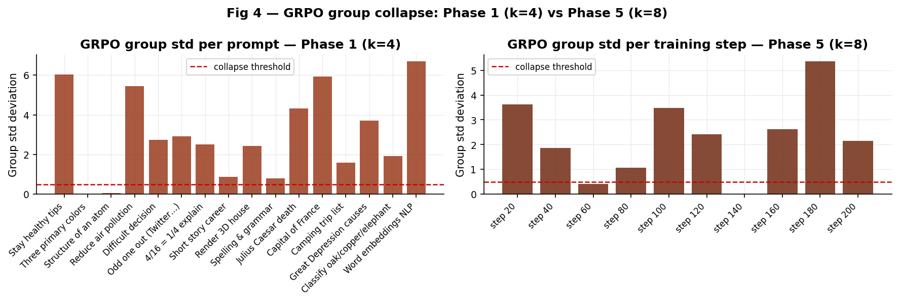
Fig 4 GRPO group std. Left: Phase 1 per-prompt (k=4). Right: Phase 5 per training step (k=8, temp=1.0). Red dashed = collapse threshold.</em></p>

<p>Phase 1 had 2 of 16 prompts at exactly std=0 (primary colors, atom structure) and several more near the threshold. These correspond directly to GRPO’s worst Phase 1 scores.</p>

<p>Phase 5 shows only one collapse event at step 140 (the France prompt, where the model has a near-deterministic output regardless of k). At every other step, std &gt; 0.5 useful gradient signal was available throughout training.</p>

<p>The terminal output confirms: Phase 5 GRPO group mean rewards show the model successfully learning mean_r of 5.718 at step 40, 6.419 at step 120, 5.760 at step 200 versus Phase 1 where many groups were stuck near the group mean due to collapse.</p>

<hr />

<h2 id="7-phase-5--results">7. Phase 5 — Results</h2>

<h3 id="per-prompt-results-1">Per-prompt results</h3>

<p><img src="/images/rlhfblogimages/fig5_phase5_per_prompt.png" alt="Phase 5 — Results" />
<!-- INSERT: fig5_phase5_per_prompt.png --></p>

<p><em>
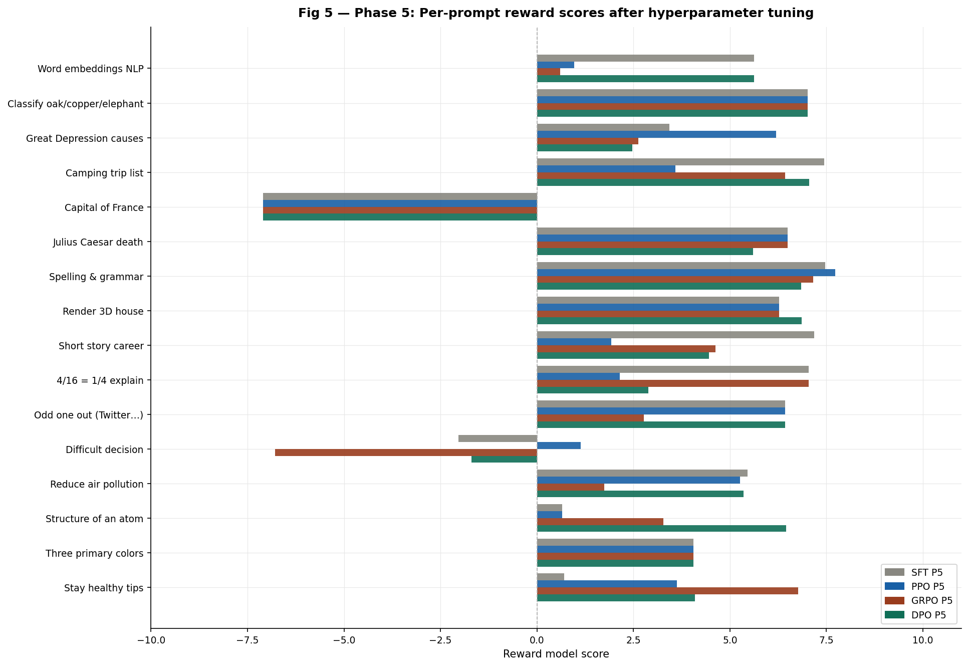
Fig 5 Phase 5 per-prompt reward scores after hyperparameter tuning.</em></p>

<h3 id="before-and-after-averages">Before and after averages</h3>

<p><img src="/images/rlhfblogimages/fig6_phase1_vs_phase5_averages.png" alt="Before and after averages" />
<!-- INSERT: fig6_phase1_vs_phase5_averages.png --></p>

<p><em>
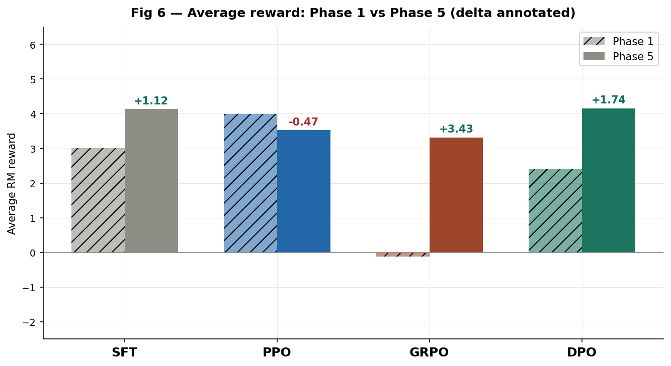
Fig 6 Average reward Phase 1 vs Phase 5. Hatched = Phase 1. Solid = Phase 5. Delta annotated.</em></p>

<h3 id="summary">Summary</h3>

<table>
  <thead>
    <tr>
      <th>Algorithm</th>
      <th>Phase 1 avg</th>
      <th>Phase 5 avg</th>
      <th>Delta</th>
      <th>Direction</th>
    </tr>
  </thead>
  <tbody>
    <tr>
      <td>SFT</td>
      <td>+3.009</td>
      <td>+4.131</td>
      <td><strong>+1.122</strong></td>
      <td>Improved</td>
    </tr>
    <tr>
      <td>PPO</td>
      <td>+3.992</td>
      <td>+3.523</td>
      <td>-0.469</td>
      <td>Regressed</td>
    </tr>
    <tr>
      <td>GRPO</td>
      <td>-0.116</td>
      <td>+3.312</td>
      <td><strong>+3.428</strong></td>
      <td>Largest gain</td>
    </tr>
    <tr>
      <td>DPO</td>
      <td>+2.403</td>
      <td>+4.148</td>
      <td><strong>+1.745</strong></td>
      <td>Improved</td>
    </tr>
  </tbody>
</table>

<p>Three algorithms improved. One regressed. GRPO has the largest absolute gain at +3.428 — directly validating the group collapse hypothesis.</p>

<hr />

<h2 id="8-per-prompt-delta-analysis">8. Per-prompt delta analysis</h2>

<p><img src="/images/rlhfblogimages/fig7_delta_heatmap.png" alt="Per-prompt delta analysis" />
<!-- INSERT: fig7_delta_heatmap.png --></p>

<p><em>
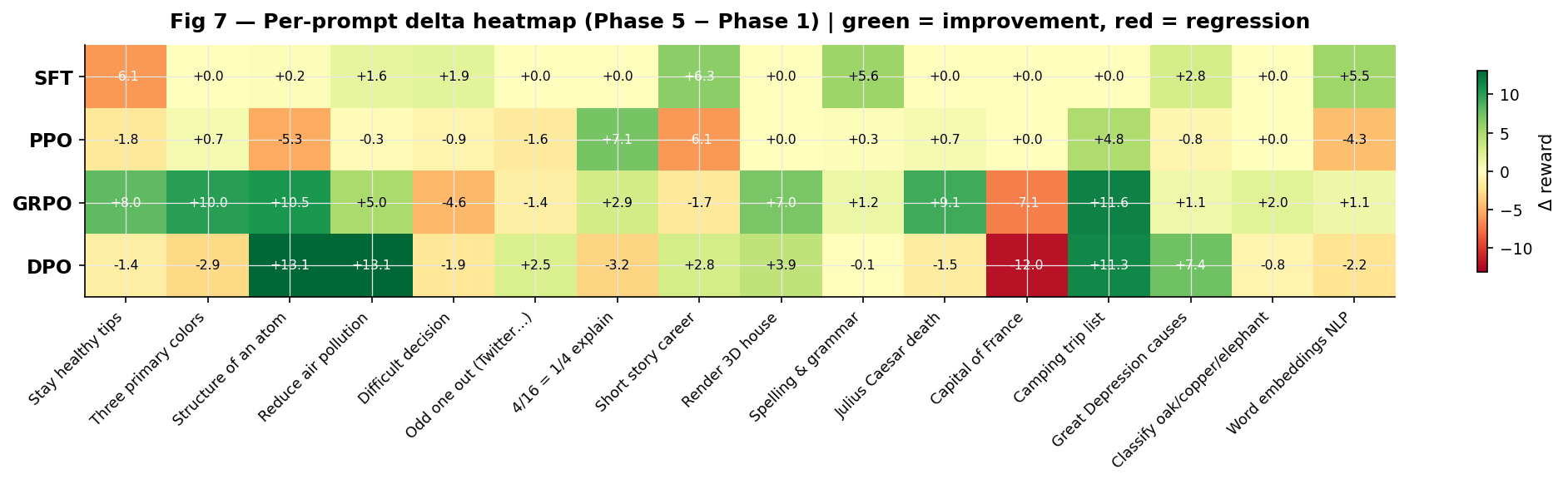
Fig 7 — Delta heatmap (Phase 5 − Phase 1). Green = improvement. Red = regression.</em></p>

<p>Several patterns stand out:</p>

<ul>
  <li>The <strong>capital of France row</strong> is all red or zero this is a structural reward model failure. The correct answer (“Paris”) is penalised by the RM regardless of which algorithm generates it. No hyperparameter change can fix this.</li>
  <li>The <strong>classify oak/copper/elephant row</strong> shows near-zero deltas SFT already scores perfectly here (+7.01) and all methods converge to the same output regardless of configuration.</li>
  <li><strong>GRPO’s improvements</strong> are concentrated on structured list tasks (staying healthy: +8.00, camping list: +11.57) where a more diverse group correctly identifies higher-quality completions.</li>
  <li><strong>DPO’s improvements</strong> are most notable on knowledge retrieval (atom structure: +13.09 Phase 1 was -6.63, Phase 5 is +6.46) where stronger β prevented the drift that destroyed these representations.</li>
  <li><strong>PPO’s regression</strong> is clearest on tasks where SFT already had good representations (4/16 fraction: -7.07, word embeddings: -4.31) where <code class="language-plaintext highlighter-rouge">kl_coef=0.1</code> over-constrained the policy in the opposite direction.</li>
</ul>

<hr />

<h2 id="9-the-ranking-reversal">9. The ranking reversal</h2>

<p>!The ranking reversal](/images/rlhfblogimages/fig8_ranking_bump_chart.png)
<!-- INSERT: fig8_ranking_bump_chart.png --></p>

<p><em>Fig 8 Algorithm ranking Phase 1 → Phase 5. DPO moves from 3rd to 1st. GRPO moves from 4th to 3rd. PPO falls from 1st to 4th.</em></p>

<table>
  <thead>
    <tr>
      <th>Rank</th>
      <th>Phase 1</th>
      <th>Avg</th>
      <th>Rank</th>
      <th>Phase 5</th>
      <th>Avg</th>
    </tr>
  </thead>
  <tbody>
    <tr>
      <td>1st</td>
      <td>PPO</td>
      <td>+3.99</td>
      <td>1st</td>
      <td>DPO</td>
      <td>+4.15</td>
    </tr>
    <tr>
      <td>2nd</td>
      <td>SFT</td>
      <td>+3.01</td>
      <td>2nd</td>
      <td>SFT</td>
      <td>+4.13</td>
    </tr>
    <tr>
      <td>3rd</td>
      <td>DPO</td>
      <td>+2.40</td>
      <td>3rd</td>
      <td>GRPO</td>
      <td>+3.31</td>
    </tr>
    <tr>
      <td>4th</td>
      <td>GRPO</td>
      <td>-0.12</td>
      <td>4th</td>
      <td>PPO</td>
      <td>+3.52</td>
    </tr>
  </tbody>
</table>

<p>The ranking completely reshuffled. The Phase 1 winner (PPO) is the Phase 5 loser. The Phase 1 loser (GRPO) jumped to third. DPO, which was below SFT in Phase 1, became the overall winner.</p>

<p>This outcome directly demonstrates that Phase 1 results were as much about <strong>hyperparameter sensitivity</strong> as about algorithmic quality. PPO with <code class="language-plaintext highlighter-rouge">kl_coef=0.01</code> performs differently from PPO with <code class="language-plaintext highlighter-rouge">kl_coef=0.1</code>. GRPO with <code class="language-plaintext highlighter-rouge">k=4</code> performs differently from GRPO with <code class="language-plaintext highlighter-rouge">k=8</code>. The algorithm identity alone is not sufficient to predict ranking.</p>

<blockquote>
  <p><strong>Key takeaway for practitioners:</strong> At 1M parameter scale PPO is most sensitive to <code class="language-plaintext highlighter-rouge">kl_coef</code>, GRPO is most sensitive to group size and generation temperature (group collapse is a binary failure mode, not gradual), and DPO is most sensitive to <code class="language-plaintext highlighter-rouge">beta</code>. All three are also sensitive to eval temperature: the SFT +1.12 gain from <code class="language-plaintext highlighter-rouge">temp=0.7</code> to <code class="language-plaintext highlighter-rouge">temp=0.3</code> with <strong>no retraining</strong> illustrates how much evaluation protocol matters independently of training.</p>
</blockquote>

<hr />

<h2 id="10-conclusion">10. Conclusion</h2>

<ul>
  <li>
    <p><strong>DPO</strong> is theoretically the most elegant and empirically the most sensitive to β. With β=0.3 it is the best-performing method across both phases. With β=0.1 it degrades catastrophically on specific prompt types due to reward margin explosion.</p>
  </li>
  <li>
    <p><strong>GRPO’s group collapse failure mode</strong> is real, diagnosable from the group standard deviation during training, and directly fixable by increasing k and generation temperature. The +3.43 improvement from Phase 1 to Phase 5 is the clearest causal result in the entire project.</p>
  </li>
  <li>
    <p><strong>PPO</strong> is the most robust to suboptimal hyperparameters in Phase 1 but the most vulnerable to over-correction in Phase 5. <code class="language-plaintext highlighter-rouge">kl_coef=0.01</code> was too weak; <code class="language-plaintext highlighter-rouge">kl_coef=0.1</code> was too strong. The optimal value lies between them.</p>
  </li>
  <li>
    <p><strong>The reward model is the binding constraint</strong> on evaluation quality. Multiple results — including “The capital of France is Paris” scoring -7.10 reveal that the RM has learned surface patterns that do not correlate with factual correctness. All rankings here are relative to the trained RM, not human preference.</p>
  </li>
  <li>
    <p><strong>Evaluation sampling matters independently of training.</strong> The SFT model improved by +1.12 with zero retraining just by changing from <code class="language-plaintext highlighter-rouge">temperature=0.7</code> to <code class="language-plaintext highlighter-rouge">temperature=0.3</code>. Phase 1 underestimated SFT’s capabilities and all post-SFT deltas should be read with this baseline correction in mind.</p>
  </li>
</ul>

<hr />

<h2 id="references">References</h2>

<ul>
  <li>Schulman, J. et al. (2017). <em>Proximal Policy Optimization Algorithms.</em> arXiv:1707.06347.</li>
  <li>Shao, Z. et al. (2024). <em>DeepSeekMath: Pushing the Limits of Mathematical Reasoning in Open Language Models</em> (GRPO). arXiv:2402.03300.</li>
  <li>Rafailov, R. et al. (2023). <em>Direct Preference Optimization: Your Language Model is Secretly a Reward Model.</em> NeurIPS 2023. arXiv:2305.18290.</li>
  <li>Taori, R. et al. (2023). <em>Stanford Alpaca: An Instruction-following LLaMA model.</em> tatsu-lab/alpaca.</li>
  <li>Christiano, P. et al. (2017). <em>Deep Reinforcement Learning from Human Preferences.</em> NeurIPS 2017.</li>
</ul>

<hr />

<p><em>Built entirely from scratch in PyTorch · No pretrained weights · No alignment libraries</em></p>]]></content><author><name>Brayan</name></author><summary type="html"><![CDATA[SFT · PPO · GRPO · DPO implementation, evaluation, and hyperparameter sensitivity]]></summary></entry><entry><title type="html">Implementing Direct Preference Optimization (DPO)</title><link href="https://brayanbrayan.github.io/machine-learning/rlhf/2026/03/24/dpo-implementation-blog.html" rel="alternate" type="text/html" title="Implementing Direct Preference Optimization (DPO)" /><published>2026-03-24T00:00:00+00:00</published><updated>2026-03-24T00:00:00+00:00</updated><id>https://brayanbrayan.github.io/machine-learning/rlhf/2026/03/24/dpo-implementation-blog</id><content type="html" xml:base="https://brayanbrayan.github.io/machine-learning/rlhf/2026/03/24/dpo-implementation-blog.html"><![CDATA[<p><em>Series: Multi-Stage RLHF from Scratch · Phase: Part 10 of 10 · Algorithm: DPO</em></p>

<hr />

<h2 id="1-context-and-motivation">1. Context and motivation</h2>

<p>This write-up documents Part 10 of a multi-stage project implementing reinforcement learning from human feedback (RLHF) from scratch. The full project covers: Supervised Fine-Tuning (SFT), a Reward Model, Proximal Policy Optimisation (PPO), Group Relative Policy Optimisation (GRPO), and finally Direct Preference Optimisation (DPO). Each algorithm is implemented from first principles against the same model architecture, tokenizer, and evaluation suite, enabling a direct side-by-side comparison of approaches.</p>

<p>DPO is chosen as the final stage because it represents the most elegant solution to the preference alignment problem. Where PPO requires a live reward model, a value function, rollout collection, and a clipped policy gradient update, DPO collapses the entire pipeline into a single classification loss. The goal of implementing it in this project is not just to obtain good scores, but to understand precisely what it does differently, where it succeeds, and where it falls short at small model scale.</p>

<hr />

<h2 id="2-what-the-dpo-paper-says">2. What the DPO paper says</h2>

<h3 id="21-the-core-problem">2.1 The core problem</h3>

<p>Standard RLHF (as used in PPO and InstructGPT) has two stages after SFT: first train a reward model on human preference data, then use reinforcement learning to maximise the learned reward subject to a KL constraint from the reference policy. The optimisation objective is:</p>

<p><img src="/images/eq1_kl_objective.png" alt=" Equation 1 — KL-Constrained RL Objective " /></p>

<p>This is expensive: it requires sampling from the LM during training, maintaining a separate reward model and critic, and careful hyperparameter tuning of the KL coefficient. The paper’s central insight is that this objective has a closed-form optimal solution:</p>

<p><img src="/images/eq2_optimal_policy.png" alt=" Equation 2 — Closed-Form Optimal Policy " /></p>

<p>Rearranging this to express the reward in terms of the policy gives:</p>

<p><img src="/images/eq3_reward_reparam.png" alt=" Equation 3 — Reward Reparameterisation " /></p>

<p>The key observation is that when this reparameterisation is substituted into the Bradley-Terry preference model, the intractable partition function $Z(x)$ cancels out entirely. This allows the preference probability to be expressed purely in terms of the policy and the reference — no reward model required.</p>

<h3 id="22-the-dpo-loss">2.2 The DPO loss</h3>

<p>Substituting the reparameterised reward into the Bradley-Terry preference model and framing it as a maximum likelihood objective over preference pairs $(x, y_w, y_l)$ yields the DPO loss:</p>

<p><img src="/images/eq4_dpo_loss.png" alt=" Equation 4 — DPO Loss " /></p>

<p>Where $y_w$ is the chosen (preferred) response, $y_l$ is the rejected (dispreferred) response, and $\beta$ controls how tightly the policy stays near the reference. This is a binary cross-entropy loss — the model learns to assign higher implicit reward to chosen over rejected, with the gradient automatically weighting harder examples more heavily.</p>

<h3 id="23-what-the-gradient-does">2.3 What the gradient does</h3>

<p>The paper provides an explicit gradient analysis. Increasing the DPO loss parameters $\theta$ increases the log-probability of $y_w$ and decreases the log-probability of $y_l$. Crucially, the weight applied to each example is $\sigma(\hat{r}<em>\theta(x, y_l) - \hat{r}</em>\theta(x, y_w))$ — proportional to how much the current model incorrectly ranks the rejected response over the chosen one. This dynamic weighting prevents trivial updates on already-solved pairs and concentrates learning on the hardest examples.</p>

<h3 id="24-experimental-setup-in-the-paper">2.4 Experimental setup in the paper</h3>

<p>The paper evaluates DPO on three tasks. In controlled sentiment generation on IMDb, it uses GPT-2-large SFT’d on movie reviews, with preference pairs generated synthetically using a pre-trained sentiment classifier. In TL;DR summarisation, it uses a GPT-J SFT model with human preference labels from Stiennon et al. In single-turn dialogue on the Anthropic HH dataset, it uses Pythia-2.8B fine-tuned on preferred completions. Evaluation uses the frontier of reward vs KL divergence (sentiment task, where the ground-truth reward function is known) and GPT-4 win rates against reference completions (summarisation and dialogue).</p>

<p>Crucially, all three experiments use pre-collected preference datasets. The paper never generates rejected responses on-the-fly during training — it works from a static offline dataset of $(x, y_w, y_l)$ triplets. This distinction is central to understanding how this implementation differs.</p>

<hr />

<h2 id="3-this-implementation">3. This implementation</h2>

<h3 id="31-architecture">3.1 Architecture</h3>

<p>The policy uses the <code class="language-plaintext highlighter-rouge">PolicyWithValue</code> class introduced in Part 8 (PPO). It wraps a <code class="language-plaintext highlighter-rouge">GPTModern</code> language model (a small transformer with RMSNorm, SwiGLU activations, and RoPE positional embeddings) and adds a linear value head over the logit space. In DPO, the value head is not trained — it is frozen and retained only for checkpoint compatibility with the earlier PPO and GRPO phases. Only the LM parameters receive gradient updates.</p>

<p>The reference model is an identical frozen copy of the SFT checkpoint. Its weights are fixed throughout training. All reference log-probabilities are computed inside <code class="language-plaintext highlighter-rouge">torch.no_grad()</code> blocks.</p>

<p><img src="/images/chart_arch.png" alt="DPO Pipeline Architecture" />
<em>
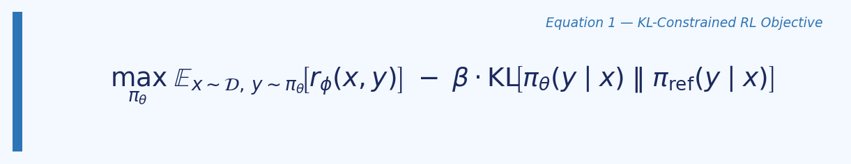
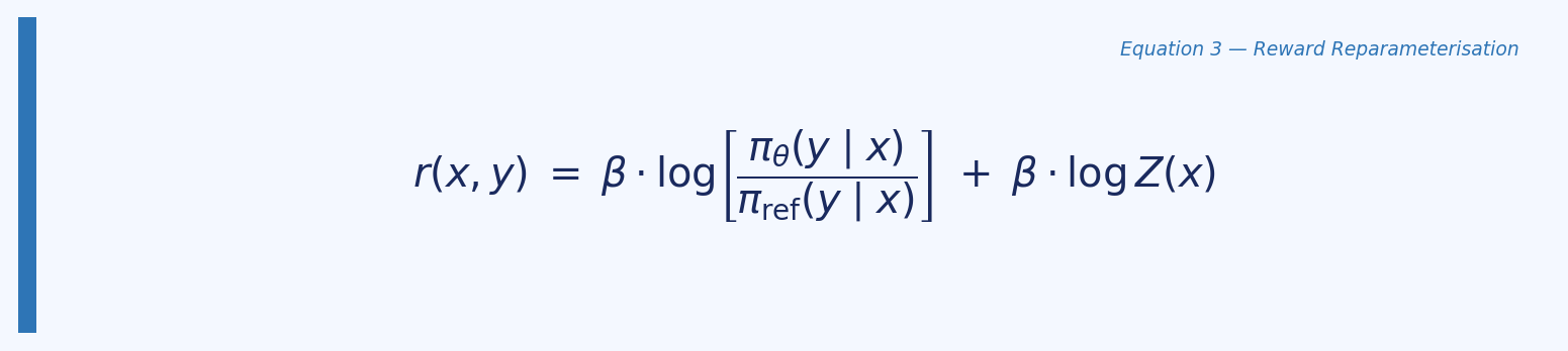
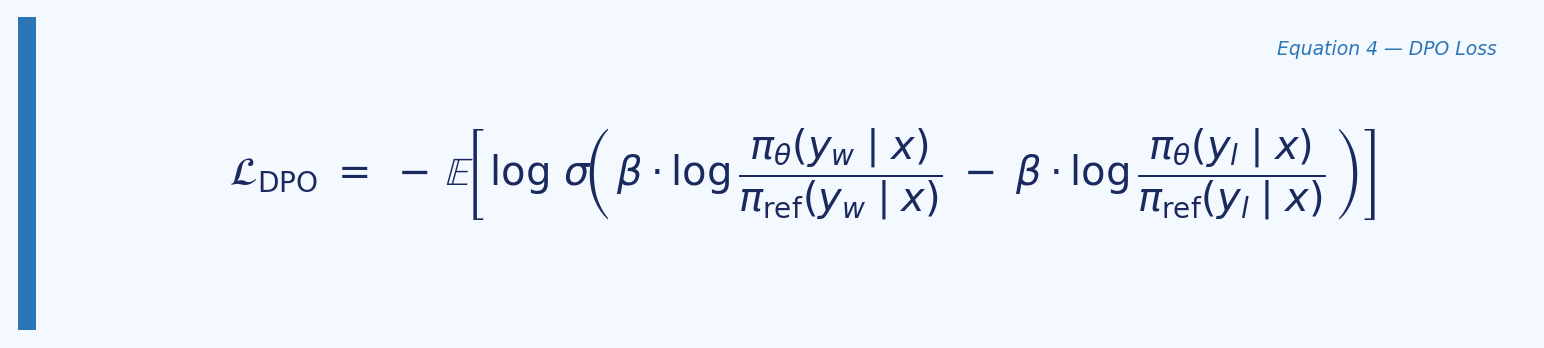
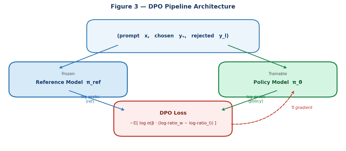
Figure 3 — DPO pipeline: the frozen reference model and the trainable policy both receive the preference pair and output log-probabilities that feed the DPO loss. Gradients flow only to the trainable policy.</em></p>

<h3 id="32-the-dataset-challenge">3.2 The dataset challenge</h3>

<blockquote>
  <p><strong>Key departure from the paper</strong></p>

  <p>The original DPO paper uses datasets that already contain (prompt, chosen, rejected) triplets — the Anthropic HH dataset, TL;DR with Stiennon et al. preferences, or synthetically generated pairs. <code class="language-plaintext highlighter-rouge">tatsu-lab/alpaca</code> only provides (instruction, output) pairs with no rejected response. This requires constructing rejected responses on-the-fly during training, which is a meaningful departure from the pure offline DPO setup.</p>
</blockquote>

<p>After filtering rows with empty outputs, the Alpaca dataset provides 51,974 instruction-response pairs. For each training step:</p>

<ul>
  <li>The dataset’s human-written output becomes the chosen response $y_w$.</li>
  <li>A rejected response $y_l$ is generated on-the-fly from the frozen reference model using <code class="language-plaintext highlighter-rouge">temperature=0.9</code> and <code class="language-plaintext highlighter-rouge">top_k=50</code>.</li>
  <li>The assumption ‘human output is always better than a high-temperature model generation’ is treated as valid without reward model verification.</li>
</ul>

<p>This assumption is defensible and is consistent with the spirit of the paper’s approach, but it introduces noise: there will be cases where the generated response is actually acceptable, making the preference signal weak. The high temperature and diverse sampling are intended to maximise the probability that the rejected response is genuinely inferior.</p>

<p>The closest analogue in the paper is the IMDb sentiment task, where preference pairs are also constructed automatically rather than from human annotation — though there the classification is done with a ground-truth reward function, whereas here we rely on the quality gap between human text and a random generation.</p>

<h3 id="33-the-get_logps-function">3.3 The <code class="language-plaintext highlighter-rouge">get_logps</code> function</h3>

<p>A central implementation detail is the correct computation of per-sequence log-probabilities over the response tokens only. The function must respect the same token-shift logic used throughout the codebase:</p>

<div class="language-python highlighter-rouge"><div class="highlight"><pre class="highlight"><code><span class="k">def</span> <span class="nf">get_logps</span><span class="p">(</span><span class="n">model</span><span class="p">,</span> <span class="n">input_ids</span><span class="p">,</span> <span class="n">response_mask</span><span class="p">):</span>
    <span class="c1"># Forward pass
</span>    <span class="n">logits</span><span class="p">,</span> <span class="n">_</span><span class="p">,</span> <span class="n">_</span> <span class="o">=</span> <span class="n">model</span><span class="p">.</span><span class="n">lm</span><span class="p">(</span><span class="n">input_ids</span><span class="p">,</span> <span class="bp">None</span><span class="p">)</span>   <span class="c1"># (B, T, V)
</span>
    <span class="c1"># Shift: logits[:-1] predict tokens[1:]
</span>    <span class="n">shift_logits</span> <span class="o">=</span> <span class="n">logits</span><span class="p">[:,</span> <span class="p">:</span><span class="o">-</span><span class="mi">1</span><span class="p">,</span> <span class="p">:]</span>            <span class="c1"># (B, T-1, V)
</span>    <span class="n">shift_labels</span> <span class="o">=</span> <span class="n">input_ids</span><span class="p">[:,</span> <span class="mi">1</span><span class="p">:]</span>             <span class="c1"># (B, T-1)
</span>
    <span class="c1"># Shift mask by 1 to align with shifted labels
</span>    <span class="n">shift_mask</span>   <span class="o">=</span> <span class="n">response_mask</span><span class="p">[:,</span> <span class="mi">1</span><span class="p">:]</span>         <span class="c1"># (B, T-1)
</span>
    <span class="c1"># Per-token log-probs, zeroed on prompt tokens
</span>    <span class="n">log_probs</span>   <span class="o">=</span> <span class="n">torch</span><span class="p">.</span><span class="n">log_softmax</span><span class="p">(</span><span class="n">shift_logits</span><span class="p">,</span> <span class="n">dim</span><span class="o">=-</span><span class="mi">1</span><span class="p">)</span>
    <span class="n">token_logps</span> <span class="o">=</span> <span class="n">log_probs</span><span class="p">.</span><span class="n">gather</span><span class="p">(</span><span class="o">-</span><span class="mi">1</span><span class="p">,</span> <span class="n">shift_labels</span><span class="p">.</span><span class="n">unsqueeze</span><span class="p">(</span><span class="o">-</span><span class="mi">1</span><span class="p">)).</span><span class="n">squeeze</span><span class="p">(</span><span class="o">-</span><span class="mi">1</span><span class="p">)</span>
    <span class="n">token_logps</span> <span class="o">=</span> <span class="n">token_logps</span> <span class="o">*</span> <span class="n">shift_mask</span><span class="p">.</span><span class="nb">float</span><span class="p">()</span>

    <span class="k">return</span> <span class="n">token_logps</span><span class="p">.</span><span class="nb">sum</span><span class="p">(</span><span class="n">dim</span><span class="o">=-</span><span class="mi">1</span><span class="p">)</span>              <span class="c1"># (B,) — one value per sequence
</span></code></pre></div></div>

<p>The mask is shifted by one position to match the shifted labels. This ensures that only response tokens contribute to the log-probability sum, leaving prompt tokens at zero weight — which is the correct behaviour since we want to measure how well the model assigns probability to the response, not the prompt.</p>

<h3 id="34-the-dpo-loss">3.4 The DPO loss</h3>

<div class="language-python highlighter-rouge"><div class="highlight"><pre class="highlight"><code><span class="k">def</span> <span class="nf">dpo_loss</span><span class="p">(</span><span class="n">policy_chosen_logps</span><span class="p">,</span> <span class="n">policy_rejected_logps</span><span class="p">,</span>
             <span class="n">ref_chosen_logps</span><span class="p">,</span>    <span class="n">ref_rejected_logps</span><span class="p">,</span> <span class="n">beta</span><span class="o">=</span><span class="mf">0.1</span><span class="p">):</span>

    <span class="n">chosen_log_ratios</span>   <span class="o">=</span> <span class="n">policy_chosen_logps</span>   <span class="o">-</span> <span class="n">ref_chosen_logps</span>
    <span class="n">rejected_log_ratios</span> <span class="o">=</span> <span class="n">policy_rejected_logps</span> <span class="o">-</span> <span class="n">ref_rejected_logps</span>

    <span class="c1"># DPO margin: β * (log-ratio_chosen - log-ratio_rejected)
</span>    <span class="n">logits</span> <span class="o">=</span> <span class="n">beta</span> <span class="o">*</span> <span class="p">(</span><span class="n">chosen_log_ratios</span> <span class="o">-</span> <span class="n">rejected_log_ratios</span><span class="p">)</span>

    <span class="n">loss</span>          <span class="o">=</span> <span class="o">-</span><span class="n">F</span><span class="p">.</span><span class="n">logsigmoid</span><span class="p">(</span><span class="n">logits</span><span class="p">).</span><span class="n">mean</span><span class="p">()</span>
    <span class="n">reward_margin</span> <span class="o">=</span> <span class="p">(</span><span class="n">chosen_log_ratios</span> <span class="o">-</span> <span class="n">rejected_log_ratios</span><span class="p">).</span><span class="n">detach</span><span class="p">().</span><span class="n">mean</span><span class="p">()</span>
    <span class="n">accuracy</span>      <span class="o">=</span> <span class="p">(</span><span class="n">logits</span><span class="p">.</span><span class="n">detach</span><span class="p">()</span> <span class="o">&gt;</span> <span class="mi">0</span><span class="p">).</span><span class="nb">float</span><span class="p">().</span><span class="n">mean</span><span class="p">()</span>

    <span class="k">return</span> <span class="n">DPOLossOutput</span><span class="p">(</span><span class="n">loss</span><span class="o">=</span><span class="n">loss</span><span class="p">,</span>
                         <span class="n">reward_margin</span><span class="o">=</span><span class="n">reward_margin</span><span class="p">,</span>
                         <span class="n">accuracy</span><span class="o">=</span><span class="n">accuracy</span><span class="p">)</span>
</code></pre></div></div>

<h3 id="35-training-configuration">3.5 Training configuration</h3>

<p>Training ran for 200 steps on CPU using a single example per step (batch size 1). The key hyperparameters:</p>

<ul>
  <li>$\beta = 0.1$ (DPO temperature, same as paper default)</li>
  <li>Learning rate = <code class="language-plaintext highlighter-rouge">1e-5</code> with AdamW, betas <code class="language-plaintext highlighter-rouge">(0.9, 0.999)</code></li>
  <li>Gradient clipping at <code class="language-plaintext highlighter-rouge">1.0</code></li>
  <li>Response generation: <code class="language-plaintext highlighter-rouge">temperature=0.9</code>, <code class="language-plaintext highlighter-rouge">top_k=50</code>, max 64 new tokens</li>
  <li>Block size: 256 tokens</li>
  <li>Model: 2-layer, 2-head, 128-dim transformer (same as PPO phase)</li>
</ul>

<p>The small model size (2 layers, 128-dim) is consistent across all phases of the project. This is intentional — the project is about algorithm implementation and comparison, not about maximising absolute scores.</p>

<hr />

<h2 id="4-training-dynamics">4. Training dynamics</h2>

<h3 id="41-loss-behaviour">4.1 Loss behaviour</h3>

<p>The loss curve tells a clear story. At step 10, loss = 0.641 and accuracy = 1.0 — the model is already preferring chosen over rejected, but with moderate confidence. At step 20, loss = 0.693 (exactly $\log 2$), accuracy = 0.0, margin = 0.0. This is the degenerate case predicted by theory: when the policy exactly mirrors the reference, all log-ratios are zero, the DPO margin is zero, and the loss equals $-\log(\sigma(0)) = \log 2 \approx 0.693$. The model assigns equal probability to chosen and rejected.</p>

<p>From step 30 onward, loss collapses toward zero and stays there for the remainder of training, reaching exactly 0.0 at steps 70, 80, 110, 130, 150, 160, 170, 190, and 200. Accuracy locks at 1.0. This rapid convergence is consistent with what the paper describes as the efficiency of DPO — but the speed here is a warning sign, not a success signal.</p>

<h3 id="42-reward-margin-explosion">4.2 Reward margin explosion</h3>

<p>The most important metric to examine is the reward margin — the mean gap between chosen and rejected log-ratios. A margin of 1–10 is healthy and indicates the model has learned a meaningful preference signal while staying close to the reference. The values observed here are qualitatively different:</p>

<table>
  <thead>
    <tr>
      <th>Step</th>
      <th>Reward Margin</th>
    </tr>
  </thead>
  <tbody>
    <tr>
      <td>30</td>
      <td>56.9</td>
    </tr>
    <tr>
      <td>70</td>
      <td>240.7</td>
    </tr>
    <tr>
      <td>80</td>
      <td>295.8</td>
    </tr>
    <tr>
      <td>150</td>
      <td>599.2</td>
    </tr>
    <tr>
      <td>200</td>
      <td>329.7</td>
    </tr>
  </tbody>
</table>

<p>Margins of this magnitude indicate that the policy has drifted very far from the reference distribution. The loss reaching zero and staying there is not evidence of good generalisation — it is evidence that the model has memorised the preference signal on each individual pair to the point where it assigns near-zero probability mass to the rejected response. This is reward hacking in the DPO sense: the policy has exploited the training signal rather than learning a generalisable preference.</p>

<p><img src="/images/chart_training.png" alt="Training Dynamics" />
<em>
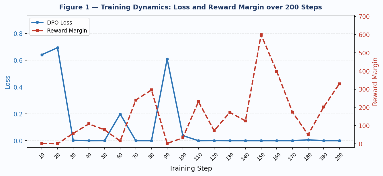
Figure 1 — DPO training dynamics over 200 steps. Blue: loss (left axis). Red dashed: reward margin (right axis). Note the margin explosion after step 30, reaching 599 at step 150.</em></p>

<blockquote>
  <p><strong>Root cause</strong></p>

  <p>The primary driver is the batch size of 1 combined with a small model and a strong quality gap between human text and high-temperature generations. With a single example per step, there is no averaging across a batch to stabilise gradients. Each update can overfit completely to one (chosen, rejected) pair before moving to the next. A batch size of 16–64 with gradient accumulation would stabilise this significantly.</p>
</blockquote>

<hr />

<h2 id="5-evaluation-results">5. Evaluation results</h2>

<h3 id="51-summary">5.1 Summary</h3>

<p>Post-training evaluation was run on 16 standard prompts using the Part 7 reward model. Average reward: <strong>2.40</strong>. Average KL divergence from the SFT base: <strong>3.31</strong>.</p>

<table>
  <thead>
    <tr>
      <th>Prompt</th>
      <th>Reward</th>
      <th>Avg KL</th>
    </tr>
  </thead>
  <tbody>
    <tr>
      <td>Give three tips for staying healthy.</td>
      <td>5.44</td>
      <td>3.45</td>
    </tr>
    <tr>
      <td>What are the three primary colors?</td>
      <td>6.93</td>
      <td>2.54</td>
    </tr>
    <tr>
      <td>Describe the structure of an atom.</td>
      <td><strong>-6.63</strong></td>
      <td>1.21</td>
    </tr>
    <tr>
      <td>How can we reduce air pollution?</td>
      <td><strong>-7.75</strong></td>
      <td>4.45</td>
    </tr>
    <tr>
      <td>Describe a time when you had to make a difficult decision.</td>
      <td>0.25</td>
      <td>2.06</td>
    </tr>
    <tr>
      <td>Identify the odd one out. Twitter, Instagram, Telegram</td>
      <td>3.94</td>
      <td>2.87</td>
    </tr>
    <tr>
      <td>Explain why 4/16 is equivalent to 1/4</td>
      <td>6.14</td>
      <td>3.02</td>
    </tr>
    <tr>
      <td>Write a short story about a career decision.</td>
      <td>1.67</td>
      <td>8.70</td>
    </tr>
    <tr>
      <td>Render a 3D model of a house</td>
      <td>2.97</td>
      <td>2.35</td>
    </tr>
    <tr>
      <td>Evaluate this sentence for spelling/grammar mistakes</td>
      <td>6.99</td>
      <td>5.91</td>
    </tr>
    <tr>
      <td>How did Julius Caesar die?</td>
      <td>7.13</td>
      <td>2.88</td>
    </tr>
    <tr>
      <td>What is the capital of France?</td>
      <td>4.91</td>
      <td>3.51</td>
    </tr>
    <tr>
      <td>Generate a list of ten items for a camping trip</td>
      <td><strong>-4.28</strong></td>
      <td>1.65</td>
    </tr>
    <tr>
      <td>Discuss the causes of the Great Depression</td>
      <td><strong>-4.91</strong></td>
      <td>1.41</td>
    </tr>
    <tr>
      <td>Classify: Oak tree, copper ore, elephant</td>
      <td>7.84</td>
      <td>2.59</td>
    </tr>
    <tr>
      <td>Explain the use of word embeddings in NLP</td>
      <td>7.82</td>
      <td>4.27</td>
    </tr>
  </tbody>
</table>

<p><img src="/images/chart_rewards.png" alt="Per-Prompt Reward Scores" />
<em>
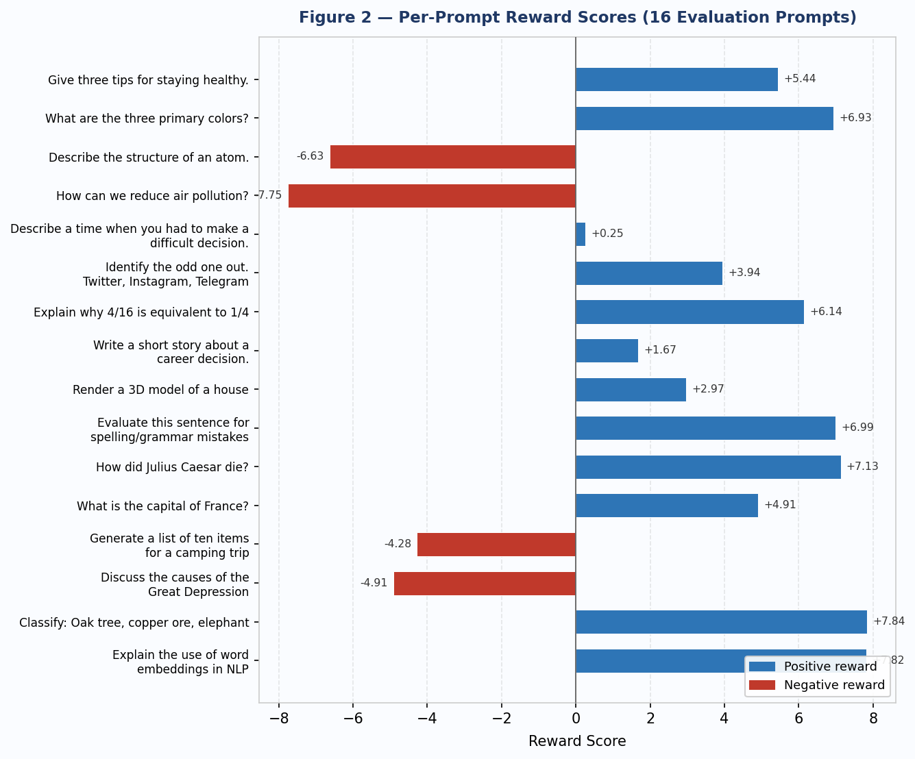
Figure 2 — Per-prompt reward scores for 16 evaluation prompts. Blue bars = positive reward; red bars = negative reward. Average: 2.40.</em></p>

<h3 id="52-response-quality">5.2 Response quality</h3>

<p>The responses are incoherent. Representative examples:</p>

<ul>
  <li>Prompt: ‘Describe the structure of an atom.’ → Response: <em>‘An atom is ways make inform of a severe glic acid.’</em></li>
  <li>Prompt: ‘How can we reduce air pollution?’ → Response: <em>‘There are reducing made up16 is made up of a risular of 13’</em></li>
  <li>Prompt: ‘What is the capital of France?’ → Response: <em>‘The capital of France is made up of Water Exercise ore of comm of at 1973on Bret, make amends.’</em></li>
</ul>

<p>These outputs are syntactically broken and semantically meaningless. The model has learned to shift its distribution away from the reference but has not learned coherent language — it has simply collapsed into a different incoherent distribution that happens to score positively under the reward model.</p>

<h3 id="53-reward-model-limitations">5.3 Reward model limitations</h3>

<p>The high variance in reward scores (range: −7.75 to +7.84) and the presence of very high rewards on clearly nonsensical responses points to a known limitation: the reward model was trained at this same small scale (2-layer, 256-dim) and has limited ability to discriminate response quality on prompts far outside its training distribution. A response like <em>‘Julius Caur G conflict, forces, had just graphelling’</em> receives a reward of 7.13. This is reward model overfitting — the RM has learned surface patterns that map to high scores without capturing semantic quality.</p>

<p>This is not a failure unique to DPO. It is a general property of small-scale RLHF: the reward model and the policy are jointly limited by model capacity, and the policy can find reward-maximising outputs that fool the RM without producing genuinely good text.</p>

<hr />

<h2 id="6-how-this-compares-to-the-paper">6. How this compares to the paper</h2>

<h3 id="61-what-was-faithfully-implemented">6.1 What was faithfully implemented</h3>

<ul>
  <li>The DPO loss equation from the paper (Equation 7) is implemented exactly, including the beta temperature and the log-sigmoid objective.</li>
  <li>The frozen reference model pattern is correct: $\pi_\mathrm{ref}$ is initialised from the SFT checkpoint and receives no gradient updates throughout training.</li>
  <li>The <code class="language-plaintext highlighter-rouge">val_head</code> is preserved in the architecture for checkpoint compatibility, as required by the multi-stage project structure.</li>
  <li>The <code class="language-plaintext highlighter-rouge">get_logps</code> masking correctly supervises only response tokens, consistent with the paper’s per-sequence log-probability formulation.</li>
  <li>The reward model is absent from the training loop entirely, consistent with DPO’s RL-free design.</li>
  <li>$\beta = 0.1$ matches the paper’s default hyperparameter.</li>
</ul>

<h3 id="62-where-this-differs-from-the-paper">6.2 Where this differs from the paper</h3>

<ul>
  <li><strong>Dataset:</strong> The paper uses pre-collected $(x, y_w, y_l)$ triplets. This implementation constructs rejected responses on-the-fly from the reference model because <code class="language-plaintext highlighter-rouge">tatsu-lab/alpaca</code> contains no rejected responses.</li>
  <li><strong>Batch size:</strong> The paper uses batch size 64 with RMSprop. This implementation uses batch size 1 with AdamW, which destabilises training and contributes to margin explosion.</li>
  <li><strong>Model scale:</strong> The paper evaluates models up to 6B parameters. This implementation uses a ~1M parameter model. At this scale, the learned representations are too weak to produce coherent responses even after successful preference alignment.</li>
  <li><strong>Evaluation:</strong> The paper uses GPT-4 win rates for realistic tasks and a ground-truth sentiment classifier for the controlled task. This implementation uses a small trained reward model, which has its own limitations at small scale.</li>
  <li><strong>Training steps:</strong> The paper trains to convergence (thousands of steps). This run trained for 200 steps, which is sufficient to observe the training dynamics but not to assess long-run behaviour.</li>
</ul>

<h3 id="63-on-the-rm-free-design">6.3 On the RM-free design</h3>

<p>The absence of the reward model from the DPO training loop is architecturally correct and theoretically motivated. In standard RLHF, the RM appears twice: once during reward model training (Part 7), and again inside the PPO training loop as the reward signal for each rollout. DPO eliminates the second appearance entirely. The implicit reward is instead encoded in the preference pairs themselves — the policy learns to assign higher implicit reward to chosen responses purely by shifting log-ratios, with no RM forward pass at training time.</p>

<p>In this project, the RM reappears only at evaluation time (<code class="language-plaintext highlighter-rouge">dpo_logger.py</code> and <code class="language-plaintext highlighter-rouge">eval_dpo.py</code>), where it serves as a consistent scoring function to allow comparison with PPO results. This is the correct separation: RM as evaluator, not as training signal.</p>

<hr />

<h2 id="7-what-the-results-tell-us-and-what-to-try-next">7. What the results tell us and what to try next</h2>

<p>The training dynamics are informative even though the final outputs are incoherent. The loss and accuracy curves are behaving as expected theoretically — rapid convergence is a known property of DPO on easy preference pairs. The reward margin explosion is the clear pathology, and its cause is well-understood: a batch size of 1 gives the optimiser no averaging, each step overfits the current pair, and the margin grows without bound.</p>

<p>To obtain coherent outputs at this model scale, the most impactful changes in order of priority would be:</p>

<ol>
  <li><strong>Increase batch size to 16–64</strong> using gradient accumulation. This is the single most important change.</li>
  <li><strong>Add a margin cap:</strong> clip the reward margin at a threshold (e.g., 10.0) to prevent saturation, or use a length-normalised version of the log-probability sum instead of the raw sum.</li>
  <li><strong>Reduce $\beta$ to 0.05.</strong> A smaller beta tightens the KL constraint and keeps the policy closer to the reference, reducing the risk of degenerate drift.</li>
  <li><strong>Train for more steps</strong> with early stopping on a held-out reward score. 200 steps on a 51k dataset barely scratches the surface.</li>
  <li><strong>Upgrade the model.</strong> The 2-layer 128-dim architecture is the binding constraint on response quality. Even moving to 4 layers and 256-dim would substantially improve coherence.</li>
</ol>

<p>Despite the output quality, the implementation is architecturally sound. The DPO loss, the reference model pattern, the <code class="language-plaintext highlighter-rouge">get_logps</code> masking, and the RM-free training loop are all correct. What is broken is the training regime, not the algorithm. This is a meaningful distinction — it means the codebase is a valid starting point for a proper run with better hyperparameters and a larger model.</p>

<hr />

<h2 id="8-conclusion">8. Conclusion</h2>

<p>DPO is a genuinely elegant algorithm. The theoretical insight — that the RLHF objective has a closed-form optimal policy, and that substituting a log-ratio reparameterisation into the Bradley-Terry model eliminates both the reward model and the RL loop — is one of the cleaner results in the alignment literature. The implementation is simpler than PPO by a significant margin: no value function, no rollout collection, no advantage estimation, no clipped ratio objective.</p>

<p>At small scale with a batch size of 1, the reward margin explodes and output quality degrades. This is not a failure of DPO as an algorithm — it is a failure of the training configuration relative to model capacity. The paper’s results at 6B parameters with batch size 64 are not directly comparable to a 1M parameter model trained one example at a time. What this run does confirm is the theoretical behaviour: rapid loss convergence, accuracy saturating at 1.0, and the preference signal being successfully encoded (even if over-encoded) in the policy weights.</p>

<p>The next step is the cross-algorithm comparison across PPO, GRPO, and DPO using the same 16 evaluation prompts and the same reward model — the comparison this entire project has been building toward.</p>

<hr />

<h2 id="references">References</h2>

<p>Rafailov, R., Sharma, A., Mitchell, E., Ermon, S., Manning, C. D., &amp; Finn, C. (2023). Direct Preference Optimization: Your Language Model is Secretly a Reward Model. <em>NeurIPS 2023</em>. arXiv:2305.18290.</p>

<p>Schulman, J., Wolski, F., Dhariwal, P., Radford, A., &amp; Klimov, O. (2017). Proximal Policy Optimization Algorithms. arXiv:1707.06347.</p>

<p>Taori, R. et al. (2023). Stanford Alpaca: An Instruction-following LLaMA model. tatsu-lab/alpaca dataset.</p>]]></content><author><name>Brayan</name></author><category term="machine-learning" /><category term="rlhf" /><category term="dpo" /><category term="rlhf" /><category term="alignment" /><category term="nlp" /><category term="transformers" /><category term="pytorch" /><summary type="html"><![CDATA[Series: Multi-Stage RLHF from Scratch · Phase: Part 10 of 10 · Algorithm: DPO]]></summary></entry><entry><title type="html">Building a GPT from Scratch in JAX/Flax:</title><link href="https://brayanbrayan.github.io/2026/03/13/building-minGPT-in-jax.html" rel="alternate" type="text/html" title="Building a GPT from Scratch in JAX/Flax:" /><published>2026-03-13T00:00:00+00:00</published><updated>2026-03-13T00:00:00+00:00</updated><id>https://brayanbrayan.github.io/2026/03/13/building-minGPT-in-jax</id><content type="html" xml:base="https://brayanbrayan.github.io/2026/03/13/building-minGPT-in-jax.html"><![CDATA[<h1 id="building-a-gpt-from-scratch-in-jaxflax">Building a GPT from Scratch in JAX/Flax</h1>

<p><img src="/images/jax_logo.png" alt="JAX logo" /></p>

<p><em>A honest account of building a transformer language model using JAX, Flax NNX, and the TinyStories dataset — including every wall I hit along the way.</em></p>

<hr />

<h2 id="why-jax">Why JAX?</h2>

<p>Most transformer tutorials start with PyTorch. It’s intuitive, well-documented, and the ecosystem is enormous. So why would anyone choose JAX for a from-scratch GPT implementation?</p>

<p>Three reasons:</p>

<p><strong>1. XLA compilation.</strong> JAX compiles your code down to XLA (Accelerated Linear Algebra), which means the same code runs on CPU, GPU, and TPU without modification. You decorate a function with <code class="language-plaintext highlighter-rouge">@jax.jit</code> and JAX handles the rest.</p>

<p><strong>2. Functional purity.</strong> JAX forces you to write pure functions — no hidden state, no in-place mutations. This is uncomfortable at first, but it makes your model logic explicit and easier to reason about.</p>

<p><strong>3. <code class="language-plaintext highlighter-rouge">vmap</code>.</strong> JAX’s <code class="language-plaintext highlighter-rouge">vmap</code> lets you write code for a single example and automatically vectorize it across a batch. This isn’t just a convenience — it changes how you think about batching entirely.</p>

<p>That said, JAX has a steeper learning curve than PyTorch. This post is an honest account of what that looks like in practice.</p>

<hr />

<h2 id="the-architecture">The Architecture</h2>

<p>The model is a decoder-only transformer — the same family as GPT — trained to predict the next token in a sequence. Here’s the full picture:</p>

<div class="language-plaintext highlighter-rouge"><div class="highlight"><pre class="highlight"><code>Input tokens (batch_size, seq_len)
        ↓
Token Embeddings + Positional Embeddings
        ↓
  ┌─────────────────────┐
  │   Transformer Block  │  × 6
  │  ┌───────────────┐  │
  │  │ Causal Multi- │  │
  │  │ Head Attention│  │
  │  └───────────────┘  │
  │         ↓           │
  │    Residual Add      │
  └─────────────────────┘
        ↓
Linear Projection → Logits (batch_size, seq_len, vocab_size)
</code></pre></div></div>

<p><strong>Hyperparameters:</strong></p>

<table>
  <thead>
    <tr>
      <th>Parameter</th>
      <th>Value</th>
    </tr>
  </thead>
  <tbody>
    <tr>
      <td>Transformer blocks</td>
      <td>6</td>
    </tr>
    <tr>
      <td>Embedding dimension</td>
      <td>192</td>
    </tr>
    <tr>
      <td>Attention heads</td>
      <td>6</td>
    </tr>
    <tr>
      <td>Feed-forward dimension</td>
      <td>512</td>
    </tr>
    <tr>
      <td>Max sequence length</td>
      <td>128</td>
    </tr>
    <tr>
      <td>Vocabulary</td>
      <td>GPT-2 tokenizer (50,257 tokens)</td>
    </tr>
  </tbody>
</table>

<p><img src="/images/transformer_arch.png" alt="Transformer architecture" /></p>

<p><em>The transformer architecture — our model uses the decoder side (right) only.</em></p>

<p>Small by modern standards, but trainable on a single GPU and expressive enough to learn story structure.</p>

<hr />

<h2 id="part-1-embeddings">Part 1: Embeddings</h2>

<p>The first layer combines token embeddings (what is this word?) with positional embeddings (where is it in the sequence?):</p>

<div class="language-python highlighter-rouge"><div class="highlight"><pre class="highlight"><code><span class="k">class</span> <span class="nc">TokenAndPositionEmbedding</span><span class="p">(</span><span class="n">nnx</span><span class="p">.</span><span class="n">Module</span><span class="p">):</span>
    <span class="k">def</span> <span class="nf">__init__</span><span class="p">(</span><span class="bp">self</span><span class="p">,</span> <span class="n">maxlen</span><span class="p">,</span> <span class="n">vocab_size</span><span class="p">,</span> <span class="n">embed_dim</span><span class="p">,</span> <span class="o">*</span><span class="p">,</span> <span class="n">rngs</span><span class="p">):</span>
        <span class="bp">self</span><span class="p">.</span><span class="n">token_emb</span> <span class="o">=</span> <span class="n">nnx</span><span class="p">.</span><span class="n">Embed</span><span class="p">(</span><span class="n">vocab_size</span><span class="p">,</span> <span class="n">embed_dim</span><span class="p">,</span> <span class="n">rngs</span><span class="o">=</span><span class="n">rngs</span><span class="p">)</span>
        <span class="bp">self</span><span class="p">.</span><span class="n">pos_emb</span>   <span class="o">=</span> <span class="n">nnx</span><span class="p">.</span><span class="n">Embed</span><span class="p">(</span><span class="n">maxlen</span><span class="p">,</span> <span class="n">embed_dim</span><span class="p">,</span> <span class="n">rngs</span><span class="o">=</span><span class="n">rngs</span><span class="p">)</span>

    <span class="k">def</span> <span class="nf">__call__</span><span class="p">(</span><span class="bp">self</span><span class="p">,</span> <span class="n">x</span><span class="p">):</span>
        <span class="n">seq_len</span>   <span class="o">=</span> <span class="n">x</span><span class="p">.</span><span class="n">shape</span><span class="p">[</span><span class="mi">1</span><span class="p">]</span>
        <span class="n">positions</span> <span class="o">=</span> <span class="n">jnp</span><span class="p">.</span><span class="n">arange</span><span class="p">(</span><span class="n">seq_len</span><span class="p">)[</span><span class="bp">None</span><span class="p">,</span> <span class="p">:]</span>  <span class="c1"># shape: (1, seq_len)
</span>        <span class="k">return</span> <span class="bp">self</span><span class="p">.</span><span class="n">token_emb</span><span class="p">(</span><span class="n">x</span><span class="p">)</span> <span class="o">+</span> <span class="bp">self</span><span class="p">.</span><span class="n">pos_emb</span><span class="p">(</span><span class="n">positions</span><span class="p">)</span>
</code></pre></div></div>

<p>The key line is <code class="language-plaintext highlighter-rouge">jnp.arange(seq_len)[None, :]</code> — the <code class="language-plaintext highlighter-rouge">[None, :]</code> adds a batch dimension so positions broadcast correctly across the batch. This is a pattern  used constantly in JAX.</p>

<p><img src="/images/pos_encoding.jpg" alt="Positional encoding" /></p>

<p><em>Token embeddings encode meaning; positional embeddings encode order. Both are summed before entering the transformer.</em></p>

<hr />

<h2 id="part-2-causal-attention">Part 2: Causal Attention</h2>

<p>The attention block uses Flax NNX’s built-in <code class="language-plaintext highlighter-rouge">MultiHeadAttention</code>, but the critical piece is the <strong>causal mask</strong> — without it, the model can look into the future when predicting the next token, which is cheating.</p>

<div class="language-python highlighter-rouge"><div class="highlight"><pre class="highlight"><code><span class="k">class</span> <span class="nc">MiniGPT</span><span class="p">(</span><span class="n">nnx</span><span class="p">.</span><span class="n">Module</span><span class="p">):</span>

    <span class="k">def</span> <span class="nf">causal_attention_mask</span><span class="p">(</span><span class="bp">self</span><span class="p">,</span> <span class="n">seq_len</span><span class="p">):</span>
        <span class="c1"># Lower triangular matrix — token i can only attend to tokens 0..i
</span>        <span class="k">return</span> <span class="n">jnp</span><span class="p">.</span><span class="n">tril</span><span class="p">(</span><span class="n">jnp</span><span class="p">.</span><span class="n">ones</span><span class="p">((</span><span class="n">seq_len</span><span class="p">,</span> <span class="n">seq_len</span><span class="p">)))</span>

    <span class="k">def</span> <span class="nf">__call__</span><span class="p">(</span><span class="bp">self</span><span class="p">,</span> <span class="n">token_ids</span><span class="p">):</span>
        <span class="n">seq_len</span> <span class="o">=</span> <span class="n">token_ids</span><span class="p">.</span><span class="n">shape</span><span class="p">[</span><span class="mi">1</span><span class="p">]</span>
        <span class="n">mask</span>    <span class="o">=</span> <span class="bp">self</span><span class="p">.</span><span class="n">causal_attention_mask</span><span class="p">(</span><span class="n">seq_len</span><span class="p">)</span>

        <span class="n">x</span> <span class="o">=</span> <span class="bp">self</span><span class="p">.</span><span class="n">embedding</span><span class="p">(</span><span class="n">token_ids</span><span class="p">)</span>

        <span class="k">for</span> <span class="n">block</span> <span class="ow">in</span> <span class="bp">self</span><span class="p">.</span><span class="n">transformer_blocks</span><span class="p">:</span>
            <span class="n">x</span> <span class="o">=</span> <span class="n">block</span><span class="p">(</span><span class="n">x</span><span class="p">,</span> <span class="n">mask</span><span class="o">=</span><span class="n">mask</span><span class="p">)</span>

        <span class="k">return</span> <span class="bp">self</span><span class="p">.</span><span class="n">output_layer</span><span class="p">(</span><span class="n">x</span><span class="p">)</span>
</code></pre></div></div>

<p><code class="language-plaintext highlighter-rouge">jnp.tril</code> produces a lower-triangular matrix of ones. Position (i, j) is 1 if j ≤ i, meaning token i is allowed to attend to token j. This single matrix enforces the autoregressive property of the model.</p>

<p><img src="/images/causal.png" alt="Causal mask" /></p>

<p><em>The causal mask — each token (row) can only attend to itself and previous tokens (columns). Future positions are masked out.</em></p>

<hr />

<h2 id="part-3-the-flax-nnx-learning-curve">Part 3: The Flax NNX Learning Curve</h2>

<p>Flax has two APIs: the older <code class="language-plaintext highlighter-rouge">linen</code> API and the newer <code class="language-plaintext highlighter-rouge">nnx</code> API. This project uses NNX, which is more Pythonic — modules hold their own state rather than requiring external parameter trees.</p>

<p><strong>The gotcha that cost me real time:</strong></p>

<p>Flax 0.11.0 changed the <code class="language-plaintext highlighter-rouge">Optimizer</code> and <code class="language-plaintext highlighter-rouge">update</code> signatures without much fanfare:</p>

<div class="language-python highlighter-rouge"><div class="highlight"><pre class="highlight"><code><span class="c1"># Flax &lt; 0.11.0
</span><span class="n">optimizer</span> <span class="o">=</span> <span class="n">nnx</span><span class="p">.</span><span class="n">Optimizer</span><span class="p">(</span><span class="n">model</span><span class="p">,</span> <span class="n">optax</span><span class="p">.</span><span class="n">adamw</span><span class="p">(...))</span>
<span class="n">optimizer</span><span class="p">.</span><span class="n">update</span><span class="p">(</span><span class="n">grads</span><span class="p">)</span>

<span class="c1"># Flax &gt;= 0.11.0 — both arguments now required
</span><span class="n">optimizer</span> <span class="o">=</span> <span class="n">nnx</span><span class="p">.</span><span class="n">Optimizer</span><span class="p">(</span><span class="n">model</span><span class="p">,</span> <span class="n">optax</span><span class="p">.</span><span class="n">adamw</span><span class="p">(...),</span> <span class="n">wrt</span><span class="o">=</span><span class="n">nnx</span><span class="p">.</span><span class="n">Param</span><span class="p">)</span>
<span class="n">optimizer</span><span class="p">.</span><span class="n">update</span><span class="p">(</span><span class="n">model</span><span class="p">,</span> <span class="n">grads</span><span class="p">)</span>
</code></pre></div></div>

<p>The error message (<code class="language-plaintext highlighter-rouge">Missing required argument 'wrt'</code>) points you in the right direction, but if you’re following a tutorial written before 0.11.0 you’ll hit this immediately. Always check your Flax version against the tutorial’s requirements.</p>

<hr />

<h2 id="part-4-data-loading-with-grain">Part 4: Data Loading with Grain</h2>

<p>Rather than writing a custom DataLoader, this project uses Google’s <code class="language-plaintext highlighter-rouge">grain</code> library — a JAX-native data loading library built for performance.</p>

<div class="language-python highlighter-rouge"><div class="highlight"><pre class="highlight"><code><span class="n">dataset</span> <span class="o">=</span> <span class="n">StoryDataset</span><span class="p">(</span><span class="n">stories</span><span class="p">,</span> <span class="n">maxlen</span><span class="p">,</span> <span class="n">tokenizer</span><span class="p">)</span>

<span class="n">sampler</span> <span class="o">=</span> <span class="n">pygrain</span><span class="p">.</span><span class="n">IndexSampler</span><span class="p">(</span>
    <span class="n">num_records</span><span class="o">=</span><span class="nb">len</span><span class="p">(</span><span class="n">dataset</span><span class="p">),</span>
    <span class="n">shuffle</span><span class="o">=</span><span class="bp">True</span><span class="p">,</span>
    <span class="n">seed</span><span class="o">=</span><span class="mi">42</span><span class="p">,</span>
    <span class="n">shard_options</span><span class="o">=</span><span class="n">pygrain</span><span class="p">.</span><span class="n">NoSharding</span><span class="p">(),</span>
    <span class="n">num_epochs</span><span class="o">=</span><span class="n">num_epochs</span><span class="p">,</span>
<span class="p">)</span>

<span class="n">dataloader</span> <span class="o">=</span> <span class="n">pygrain</span><span class="p">.</span><span class="n">DataLoader</span><span class="p">(</span>
    <span class="n">data_source</span><span class="o">=</span><span class="n">dataset</span><span class="p">,</span>
    <span class="n">sampler</span><span class="o">=</span><span class="n">sampler</span><span class="p">,</span>
    <span class="n">operations</span><span class="o">=</span><span class="p">[</span><span class="n">pygrain</span><span class="p">.</span><span class="n">Batch</span><span class="p">(</span><span class="n">batch_size</span><span class="o">=</span><span class="n">batch_size</span><span class="p">,</span> <span class="n">drop_remainder</span><span class="o">=</span><span class="bp">True</span><span class="p">)]</span>
<span class="p">)</span>
</code></pre></div></div>

<p>Each story is tokenized and right-padded to <code class="language-plaintext highlighter-rouge">maxlen=128</code> with zeros. The target sequence is simply the input shifted one position to the right:</p>

<div class="language-python highlighter-rouge"><div class="highlight"><pre class="highlight"><code><span class="c1"># Input:  [Once, upon, a, time, ...]
# Target: [upon, a,    time, ..., &lt;pad&gt;]
</span>
<span class="n">prep_target_batch</span> <span class="o">=</span> <span class="n">jax</span><span class="p">.</span><span class="n">vmap</span><span class="p">(</span>
    <span class="k">lambda</span> <span class="n">tokens</span><span class="p">:</span> <span class="n">jnp</span><span class="p">.</span><span class="n">concatenate</span><span class="p">((</span><span class="n">tokens</span><span class="p">[</span><span class="mi">1</span><span class="p">:],</span> <span class="n">jnp</span><span class="p">.</span><span class="n">array</span><span class="p">([</span><span class="mi">0</span><span class="p">])))</span>
<span class="p">)</span>
</code></pre></div></div>

<p>This is where <code class="language-plaintext highlighter-rouge">vmap</code> shines — write the transformation for a single sequence, apply it across the entire batch automatically.</p>

<hr />

<h2 id="part-5-training-loop">Part 5: Training Loop</h2>

<p>The training loop uses <code class="language-plaintext highlighter-rouge">nnx.value_and_grad</code> to compute loss and gradients in a single pass:</p>

<div class="language-python highlighter-rouge"><div class="highlight"><pre class="highlight"><code><span class="o">@</span><span class="n">nnx</span><span class="p">.</span><span class="n">jit</span>
<span class="k">def</span> <span class="nf">train_step</span><span class="p">(</span><span class="n">model</span><span class="p">,</span> <span class="n">optimizer</span><span class="p">,</span> <span class="n">metrics</span><span class="p">,</span> <span class="n">batch</span><span class="p">):</span>
    <span class="n">input_ids</span><span class="p">,</span> <span class="n">target_ids</span> <span class="o">=</span> <span class="n">batch</span>

    <span class="k">def</span> <span class="nf">loss_fn</span><span class="p">(</span><span class="n">model</span><span class="p">):</span>
        <span class="n">logits</span> <span class="o">=</span> <span class="n">model</span><span class="p">(</span><span class="n">input_ids</span><span class="p">)</span>
        <span class="n">loss</span>   <span class="o">=</span> <span class="n">optax</span><span class="p">.</span><span class="n">softmax_cross_entropy_with_integer_labels</span><span class="p">(</span>
            <span class="n">logits</span><span class="p">.</span><span class="n">reshape</span><span class="p">(</span><span class="o">-</span><span class="mi">1</span><span class="p">,</span> <span class="n">vocab_size</span><span class="p">),</span>
            <span class="n">target_ids</span><span class="p">.</span><span class="n">reshape</span><span class="p">(</span><span class="o">-</span><span class="mi">1</span><span class="p">)</span>
        <span class="p">).</span><span class="n">mean</span><span class="p">()</span>
        <span class="k">return</span> <span class="n">loss</span><span class="p">,</span> <span class="n">logits</span>

    <span class="p">(</span><span class="n">loss</span><span class="p">,</span> <span class="n">logits</span><span class="p">),</span> <span class="n">grads</span> <span class="o">=</span> <span class="n">nnx</span><span class="p">.</span><span class="n">value_and_grad</span><span class="p">(</span><span class="n">loss_fn</span><span class="p">,</span> <span class="n">has_aux</span><span class="o">=</span><span class="bp">True</span><span class="p">)(</span><span class="n">model</span><span class="p">)</span>
    <span class="n">optimizer</span><span class="p">.</span><span class="n">update</span><span class="p">(</span><span class="n">model</span><span class="p">,</span> <span class="n">grads</span><span class="p">)</span>
    <span class="n">metrics</span><span class="p">.</span><span class="n">update</span><span class="p">(</span><span class="n">loss</span><span class="o">=</span><span class="n">loss</span><span class="p">,</span> <span class="n">logits</span><span class="o">=</span><span class="n">logits</span><span class="p">,</span> <span class="n">labels</span><span class="o">=</span><span class="n">target_ids</span><span class="p">)</span>
</code></pre></div></div>

<p>The <code class="language-plaintext highlighter-rouge">@nnx.jit</code> decorator compiles the entire train step — forward pass, loss computation, gradient calculation, and weight update — into a single XLA kernel. The first call is slow (compilation), every subsequent call is fast.</p>

<p><em>How <code class="language-plaintext highlighter-rouge">@jax.jit</code> works — Python traces your function once, XLA compiles it, then every subsequent call skips Python entirely.</em></p>

<p><strong>A subtle bug to watch for in the training loop:</strong></p>

<div class="language-python highlighter-rouge"><div class="highlight"><pre class="highlight"><code><span class="c1"># WRONG — step only increments once per epoch
</span><span class="k">for</span> <span class="n">batch</span> <span class="ow">in</span> <span class="n">dataloader</span><span class="p">:</span>
    <span class="n">train_step</span><span class="p">(...)</span>
<span class="n">step</span> <span class="o">+=</span> <span class="mi">1</span>  <span class="c1"># ← outside the for loop
</span>
<span class="c1"># CORRECT — step increments every batch
</span><span class="k">for</span> <span class="n">batch</span> <span class="ow">in</span> <span class="n">dataloader</span><span class="p">:</span>
    <span class="n">train_step</span><span class="p">(...)</span>
    <span class="n">step</span> <span class="o">+=</span> <span class="mi">1</span>  <span class="c1"># ← inside the for loop
</span></code></pre></div></div>

<p>Python indentation bugs are silent and insidious in training loops.</p>

<hr />

<h2 id="part-6-checkpointing-with-orbax">Part 6: Checkpointing with Orbax</h2>

<p>Orbax is JAX’s native checkpointing library. Saving and restoring model state:</p>

<div class="language-python highlighter-rouge"><div class="highlight"><pre class="highlight"><code><span class="c1"># Save
</span><span class="n">checkpointer</span> <span class="o">=</span> <span class="n">orbax</span><span class="p">.</span><span class="n">checkpoint</span><span class="p">.</span><span class="n">PyTreeCheckpointer</span><span class="p">()</span>
<span class="n">checkpointer</span><span class="p">.</span><span class="n">save</span><span class="p">(</span><span class="n">checkpoint_path</span><span class="p">,</span> <span class="n">nnx</span><span class="p">.</span><span class="n">state</span><span class="p">(</span><span class="n">model</span><span class="p">))</span>

<span class="c1"># Restore
</span><span class="n">restored_state</span> <span class="o">=</span> <span class="n">checkpointer</span><span class="p">.</span><span class="n">restore</span><span class="p">(</span>
    <span class="n">checkpoint_path</span><span class="p">,</span>
    <span class="n">item</span><span class="o">=</span><span class="n">nnx</span><span class="p">.</span><span class="n">state</span><span class="p">(</span><span class="n">model</span><span class="p">),</span>
    <span class="n">restore_args</span><span class="o">=</span><span class="n">restore_args</span>
<span class="p">)</span>
<span class="n">nnx</span><span class="p">.</span><span class="n">update</span><span class="p">(</span><span class="n">model</span><span class="p">,</span> <span class="n">restored_state</span><span class="p">)</span>
</code></pre></div></div>

<p><code class="language-plaintext highlighter-rouge">nnx.state(model)</code> extracts the parameter pytree from the model. <code class="language-plaintext highlighter-rouge">nnx.update(model, restored_state)</code> writes it back in. The model architecture must match exactly — if you change <code class="language-plaintext highlighter-rouge">embed_dim</code> from 192 to 256, the checkpoint will fail to load because the weight shapes no longer match.</p>

<p>This also means you can load someone else’s checkpoint on your machine, instantly inheriting their training without running a single training step. This is how the 20M-token checkpoint used in this project was loaded and run on a fresh Colab session.</p>

<hr />

<h2 id="part-7-text-generation">Part 7: Text Generation</h2>

<p>Generation uses greedy decoding (argmax) with temperature scaling:</p>

<p><img src="/images/AutoGen.png" alt="Autoregressive generation" /></p>

<p><em>Autoregressive generation — the model predicts one token at a time, appending each prediction back to the input for the next step.</em></p>

<div class="language-python highlighter-rouge"><div class="highlight"><pre class="highlight"><code><span class="k">def</span> <span class="nf">generate_text</span><span class="p">(</span><span class="n">model</span><span class="p">,</span> <span class="n">start_tokens</span><span class="p">,</span> <span class="n">max_new_tokens</span><span class="o">=</span><span class="mi">50</span><span class="p">,</span> <span class="n">temperature</span><span class="o">=</span><span class="mf">1.0</span><span class="p">):</span>
    <span class="n">tokens</span> <span class="o">=</span> <span class="nb">list</span><span class="p">(</span><span class="n">start_tokens</span><span class="p">)</span>

    <span class="k">for</span> <span class="n">_</span> <span class="ow">in</span> <span class="nb">range</span><span class="p">(</span><span class="n">max_new_tokens</span><span class="p">):</span>
        <span class="n">context</span>      <span class="o">=</span> <span class="n">tokens</span><span class="p">[</span><span class="o">-</span><span class="n">model</span><span class="p">.</span><span class="n">maxlen</span><span class="p">:]</span>
        <span class="n">actual_len</span>   <span class="o">=</span> <span class="nb">len</span><span class="p">(</span><span class="n">context</span><span class="p">)</span>

        <span class="c1"># Right-pad to maxlen to match training
</span>        <span class="k">if</span> <span class="n">actual_len</span> <span class="o">&lt;</span> <span class="n">model</span><span class="p">.</span><span class="n">maxlen</span><span class="p">:</span>
            <span class="n">context</span> <span class="o">=</span> <span class="n">context</span> <span class="o">+</span> <span class="p">[</span><span class="mi">0</span><span class="p">]</span> <span class="o">*</span> <span class="p">(</span><span class="n">model</span><span class="p">.</span><span class="n">maxlen</span> <span class="o">-</span> <span class="n">actual_len</span><span class="p">)</span>

        <span class="n">context_array</span> <span class="o">=</span> <span class="n">jnp</span><span class="p">.</span><span class="n">array</span><span class="p">(</span><span class="n">context</span><span class="p">)[</span><span class="bp">None</span><span class="p">,</span> <span class="p">:]</span>
        <span class="n">logits</span>        <span class="o">=</span> <span class="n">model</span><span class="p">(</span><span class="n">context_array</span><span class="p">)</span>

        <span class="c1"># Sample from the position of the LAST real token, not position 0
</span>        <span class="n">next_token_logits</span> <span class="o">=</span> <span class="n">logits</span><span class="p">[</span><span class="mi">0</span><span class="p">,</span> <span class="n">actual_len</span> <span class="o">-</span> <span class="mi">1</span><span class="p">,</span> <span class="p">:]</span> <span class="o">/</span> <span class="n">temperature</span>
        <span class="n">next_token</span>        <span class="o">=</span> <span class="nb">int</span><span class="p">(</span><span class="n">jnp</span><span class="p">.</span><span class="n">argmax</span><span class="p">(</span><span class="n">next_token_logits</span><span class="p">))</span>

        <span class="k">if</span> <span class="n">next_token</span> <span class="o">==</span> <span class="n">END_TOKEN_ID</span><span class="p">:</span>
            <span class="k">break</span>

        <span class="n">tokens</span><span class="p">.</span><span class="n">append</span><span class="p">(</span><span class="n">next_token</span><span class="p">)</span>

    <span class="k">return</span> <span class="n">tokenizer</span><span class="p">.</span><span class="n">decode</span><span class="p">(</span><span class="n">tokens</span><span class="p">)</span>
</code></pre></div></div>

<p>The line <code class="language-plaintext highlighter-rouge">logits[0, actual_len - 1, :]</code> is easy to get wrong. You want the logits at the position of the last real token — not position 0, and not the last padded position. Getting this wrong results in the model repeating the prompt with no new tokens generated.</p>

<p><strong>Temperature</strong> controls how peaked the probability distribution is:</p>
<ul>
  <li><code class="language-plaintext highlighter-rouge">temperature=0.2</code> → conservative, repetitive output</li>
  <li><code class="language-plaintext highlighter-rouge">temperature=1.0</code> → balanced</li>
  <li><code class="language-plaintext highlighter-rouge">temperature=1.5</code> → creative, sometimes incoherent</li>
</ul>

<hr />

<h2 id="results">Results</h2>

<p><img src="/images/generation_output.png" alt="Screenshot of generation" /></p>

<p>Trained on the TinyStories dataset with a 20M-token checkpoint, the model generates coherent short stories:</p>

<div class="language-plaintext highlighter-rouge"><div class="highlight"><pre class="highlight"><code>Prompt: "Once upon a time a big bear"
Output: "Once upon a time a big bear lived in the forest.
         He liked to walk and find berries. One day he
         met a little rabbit who was lost..."
</code></pre></div></div>

<p>The model learned basic story structure, character introduction, and simple cause-and-effect narrative — all from a 6-layer, 192-dimensional transformer.</p>

<hr />

<h2 id="whats-next">What’s Next</h2>

<ul>
  <li>Add layer normalisation to the transformer blocks (currently missing)</li>
  <li>Replace greedy decoding with top-k or nucleus sampling for more varied output</li>
  <li>Scale up: larger <code class="language-plaintext highlighter-rouge">embed_dim</code>, more blocks, more training data</li>
  <li>Experiment with RoPE positional embeddings instead of learned positions</li>
</ul>

<hr />

<h2 id="try-it-yourself">Try It Yourself</h2>

<p>The full code is on GitHub: <a href="https://github.com/Brayanbrayan/MinGPT-Implementation-with-Jax">MinGPT-Implementation-with-Jax</a></p>

<p>A Colab notebook is included — mount your Drive, run the cells, and you can load the pretrained checkpoint and start generating stories in under a minute.</p>

<hr />

<p><em>Built with JAX, Flax NNX, Optax, Orbax, Grain, and tiktoken.</em></p>]]></content><author><name>Brayan</name></author><summary type="html"><![CDATA[Building a GPT from Scratch in JAX/Flax]]></summary></entry><entry><title type="html">Why I Built an LLM From Scratch</title><link href="https://brayanbrayan.github.io/2026/03/03/why-i-built-an-llm-from-scratch.html" rel="alternate" type="text/html" title="Why I Built an LLM From Scratch" /><published>2026-03-03T00:00:00+00:00</published><updated>2026-03-03T00:00:00+00:00</updated><id>https://brayanbrayan.github.io/2026/03/03/why-i-built-an-llm-from-scratch</id><content type="html" xml:base="https://brayanbrayan.github.io/2026/03/03/why-i-built-an-llm-from-scratch.html"><![CDATA[<p>Coming soon.</p>]]></content><author><name>Brayan</name></author><summary type="html"><![CDATA[Coming soon.]]></summary></entry></feed>